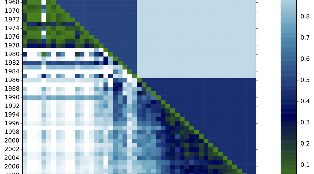
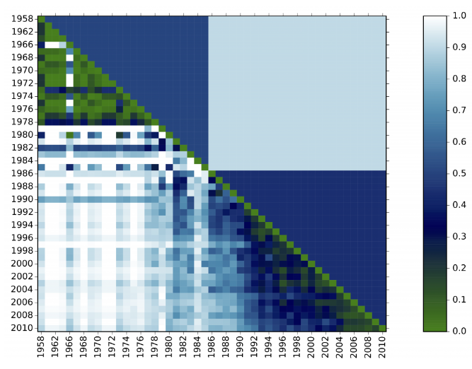
In the plot above, we see two periods detected. Every diagonal cell scores 0 because the distributions are perfectly aligned. The whiter the cell, the more dissimilar two time steps are.

Detecting periods from frequencies

Period detector directly works on the frequency distribution of one or more field to produce a matrix representing distances between the composition of the dataset for every pair of different time steps. For example, indexed by years.

For each year, the method computes a vector with the distribution of term frequencies in that year. Then, it constructs a matrix of the cosine distances between the distributions for each pair of years, corresponding to 1 minus the cosine between their vectors. It then places a fixed number of cut points along the years, producing periods, by finding the partition that minimizes the sum – over all periods – of the sum of the cosine distances between all pairs of years within each period. If the number of periods is not provided, then an optimal number is chosen according to the statistical criterion of (Tibshirani et al., 2001).

Field

This parameter defines the fields from which to construct the frequency vector distributions at each time step.

Enter the number of periods you which to detect

This parameter defines the number of periods in which to partition the data. If set to 0 (zero), the number of periods will be automatically estimated.

Top items

This parameter restrains the computation to the N most  frequent items from the selected field or fields. This may be useful as the distributions from some of the different fields may be too noisy in their lower frequencies, which would affect the distances.

What to do next?

Beyond reflecting on the matrix and the periods detected in your studies, you may want to take these results to Period Slicer and separate your dataset into custom periods.

Reference

Robert Tibshirani, Guenther Walther and Trevor Hastie, Estimating the number of clusters in a data set via the gap statistic, J.R. Statist. Soc. B (2001), 63, Part 2, pp. 411-423 (online).