The spatialization performed by CorText Manager follows the classical Fruchterman Reingold layout (Fruchterman et al. 1991). However the traditional force directed algorithm is tuned in such a way that a gravity force attracts every node toward the centroid of the cluster they belong to.

Clusters detection method: community detection algorithm

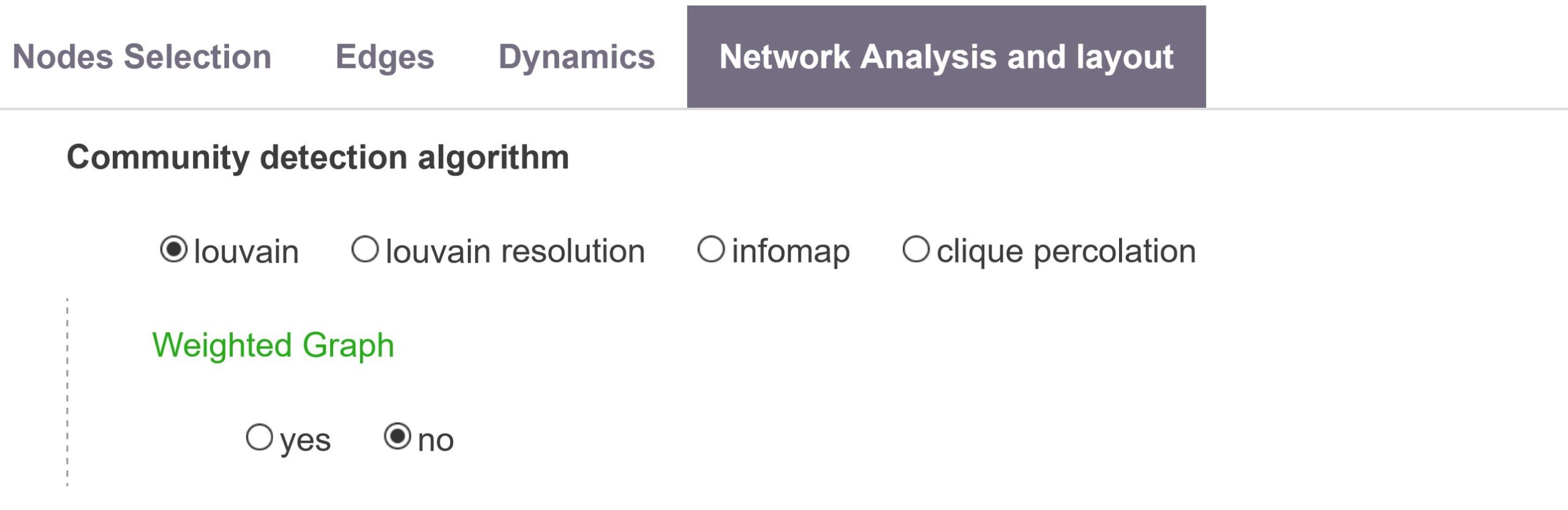
The Network Mapping script automatically identifies locally dense groups of nodes in the network. Different definitions/algorithm of these “communities of nodes” are possible. Users can choose between three popular ways to compute these meso-level structures. 

louvain resolution

When Louvain resolution (Aynaud, 2020) is chosen, users can define the Parameter resolution value (Lambiotte et al., 2008), which goes from 0.1 up to 4.9. The default value is 1 where density of the linkages inside clusters compared to the links between clusters is optimal (optimization of the “modularity” of a partition of the network). Resolution is a parameter for the Louvain community detection algorithm (Blondel et al. 2008) that affects the size of the clusters. Smaller resolutions recover smaller clusters (so, a higher number of clusters), and larger values recover clusters containing more nodes (so, a fewer number of clusters). We recommande to use louvain resolution instead of louvain (with Resolution parameter set to 1 for the defaut behaviour).

louvain

Louvain (Blondel et al. 2008) is a popular hierarchical community detection algorithm, efficent on large networks. It is based on an optimisation of the modularity, where modularity measures the density of edges within communities compared to the number of edges connecting each communities. If Weighted Graph option is Yes, it will use the louvain resolution algorithm with Resolution parameter set to 1.

infomap

Infomap (Rosvall et al. 2008), may succeed in detecting finer-grained communities.

clique percolation

Clique percolation (Palla et al. 2005), main advantage is to be interpretable as an algebraic property even though it will tend to exclude poorly connected nodes.

Historical layout

When mapping networks, two options are available to define nodes abscissa (x coordinate). By default, nodes are spatialized in 2d and take positions that optimize the stress produced by network topology (typically two nodes are attracted when connected by a link, the force being proportional to edge weight).

Historical map

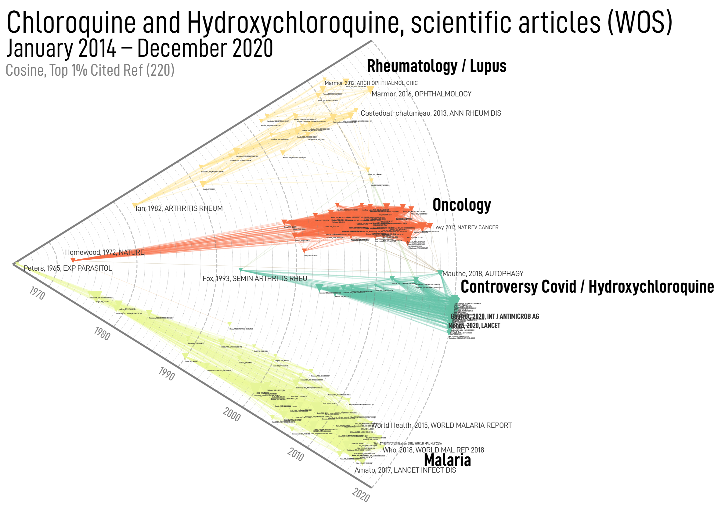
But one can also choose to fix x-position of node according to their “date”. For example, cited references will be positioned according to their publication dates – the network layout is then solely optimized according to the y-axis. This option will produce historical maps such as the one illustrated above on cited references from scientific articles published in 2020.

In other cases for which a “natural” date is not provided, historical maps are still possible but the “time” at which nodes are positioned then correspond to the date when their number of occurrences reaches 20% of their total frequency over the whole dataset.

Logarithmic scale

Nodes x-axis coordinate will still be positionned according to their birth rate with a logarithmic scale. Useful if most nodes are concentrated on a period distant from oldest nodes.

Project records onto clusters

Project records onto clusters

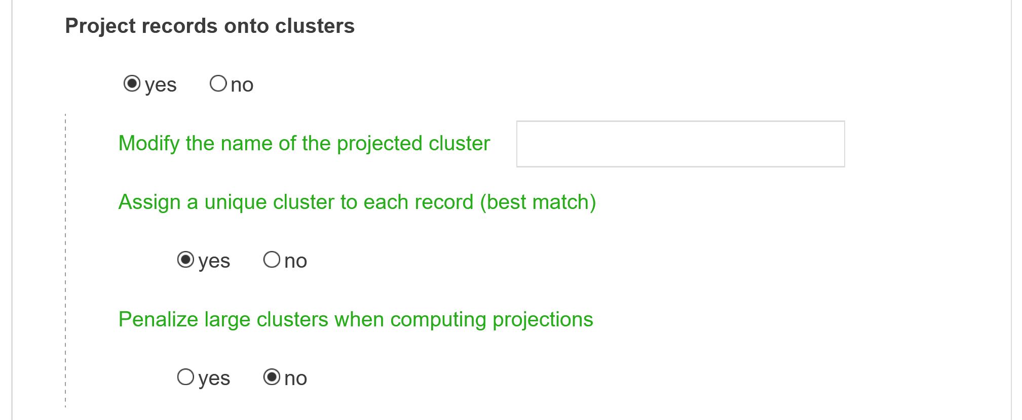
By default, once the cluster structure of the map has been determined, every article is matched against each cluster composition to assess how close their content are. A document may then be assigned to zero or several clusters at once. Additionally, a new table (whose name starts with “projection_cluster” followed by the field name) will be created in the database. This new table can be used as a new field for further analysis.

Modify the name of the projected cluster

If you do not enter anything the default name will be prefixed by projection_cluster followed by fields name.

Assign a unique cluster to each record (best match)

This option can be activated to limit the maximum number of clusters assigned to each document to 1. The most similar cluster to a given document is then selected, as long as this similarity is higher than a predetermined threshold (meaning that some documents may still stay unassigned).

Penalize large clusters when computing projections

Activate this option if you want to find former results from the first version of CorText Manager (Manager v1).

Add information from a 3rd variable

Choose the new field that should be used

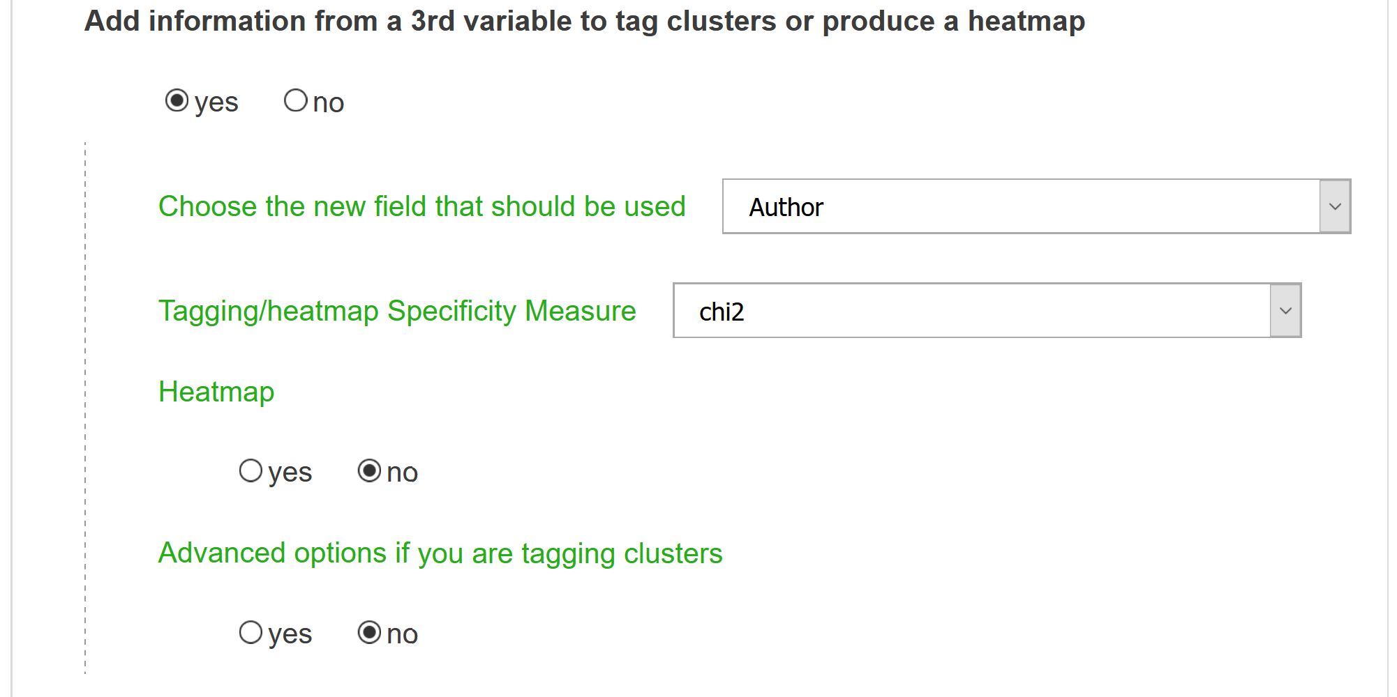
This option will produce tags associated to each cluster according to a new dimension in the dataset. It will also activate the ability to compute a heatmap from specific values of the chosen third variable.

Tagging/heatmap Specificity Measure

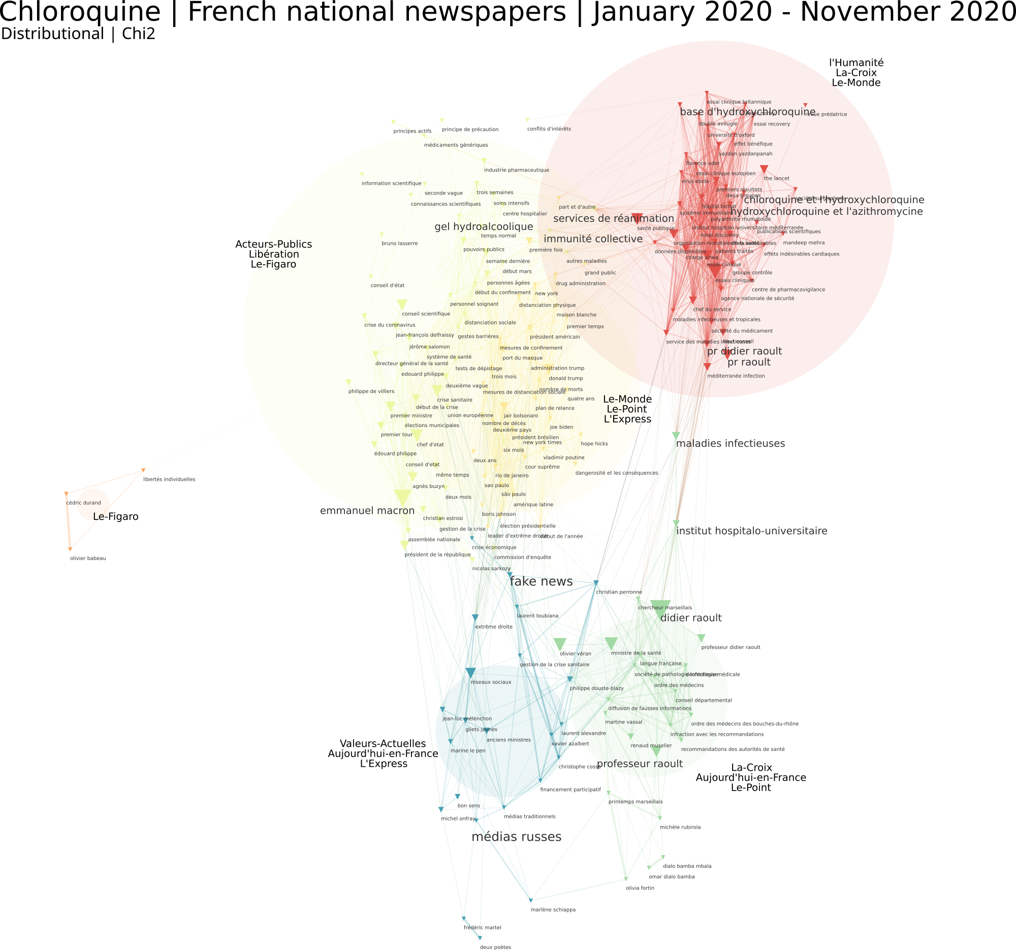
A tagging metric should be chosen. Only top N closest tags will appear on the final map (N being an option to be defined in the form). Tagging option is equivalent to computing a new network onto the different clusters that have been identified. Put differently, an heterogeneous network is computed between the cluster field and a second chosen one. For instance, one can compute a journal co-citation network and then tag them with Newspaper names (see illustration below). Articles are then projected onto these clusters which become a new kind of variable (field 1). A proximity network between those semantic clusters and entities field used for tagging can then be computed. Options are tf (for “Term Frequency”: global frequency of the entity), raw (number of times the entity appear in each cluster), chi2 (a chi2 proximity measure is computed between semantic clusters and tagged entities), cramer, mutual information (see the full description of metrics for more information). The distinction between tf and raw for tagged entities, is close to the two ways to calculate the proportions of each node in the coocurrences network (see: Nodes weight parameter in Node selection page). Other metrics proposed are rather designed for heatmaps (see below: metrics for heatmaps).

Heatmap

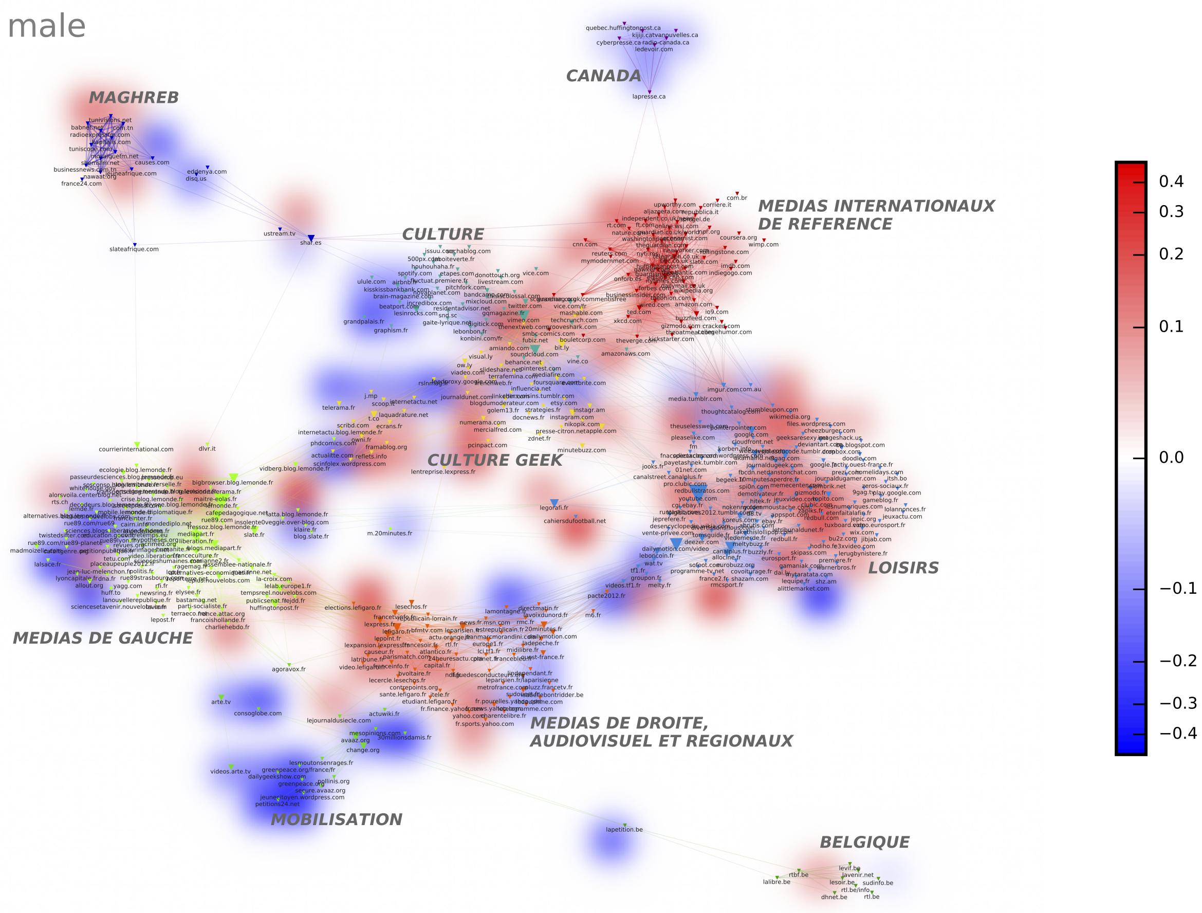
Heatmaps allow to overlay on a given network (let’s say a co-citation network on Facebook: domains are linked when they are oftentimes being shared by the same users) the distribution of presence of an entity taken from a different field (for example the gender of the Facebook user). Both the new field and the variable have to be indicated (in our case male). The algorithm computes for every node on the map its specificity with this modality: are men more likely to share links about 9gag.tv ? Possible metrics are the same than the one available for tagging clusters, plus chi2_dir, cramer_dir and cooc_deviation which are more useful in this setting. Chi2_dir and Cramer_dir correspond to the classic chi2 and cramer measures except they will also allow the user to observe negative correlations, generating a blue area in the final visualization. Cooc_deviation also measures how distant the number of citations of 9gag.tv by men is from what it should have been if this domain was uniformly distributed among men and women (relatively to their respective numbers). If positive let’s say 2: this means that the number of citations by men is twice what should be expected. If negative let’s say – 2: it means twice the number of citations of 9gag.tv by men would have been needed to reach its expected theoretical number. The final visualisation averages the different specificity scores measured at each point of the network to produce a heatmap.

Value of the field you wish to plot the heatmap of

Write the specific value you want to represent as a heatmap. It is case sensitive. In the example below “male” as been plotted and positioned on the map using the chi2-dir strategy.

Choose a period length for a dynamic profiling of the projected entity

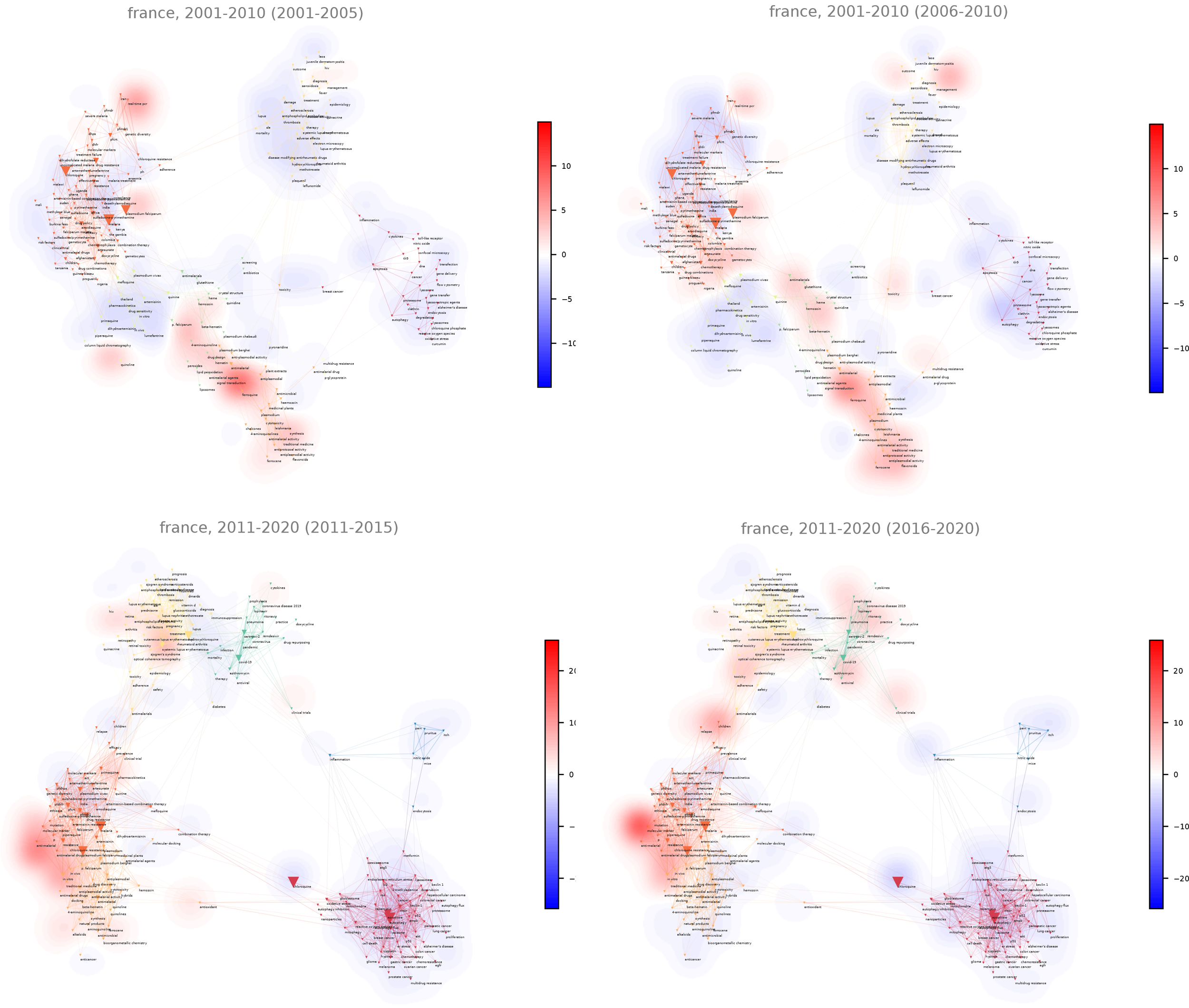
Note finally that you can compute heatmaps over time. The background map will not change and shall still depend on the dynamical settings set in Dynamical settings panel (see: “Define time periods” parameter). But the distribution of the variable plotted on the heatmap will depend on the time range you chose (one needs to define a time period over which successive heatmaps will be computed).

For instance, with a corpus which covers 2001 to 2020, choose 2 regular time periods (Number of time slices) in the Dynamical settings panel, and define the parameter “Choose a period length for a dynamic profiling of the projected entity” as 2: it will automatically produce a set of 4 maps of five years (so with two distinct background maps, one for each period).

Network analysis layout advanced settings

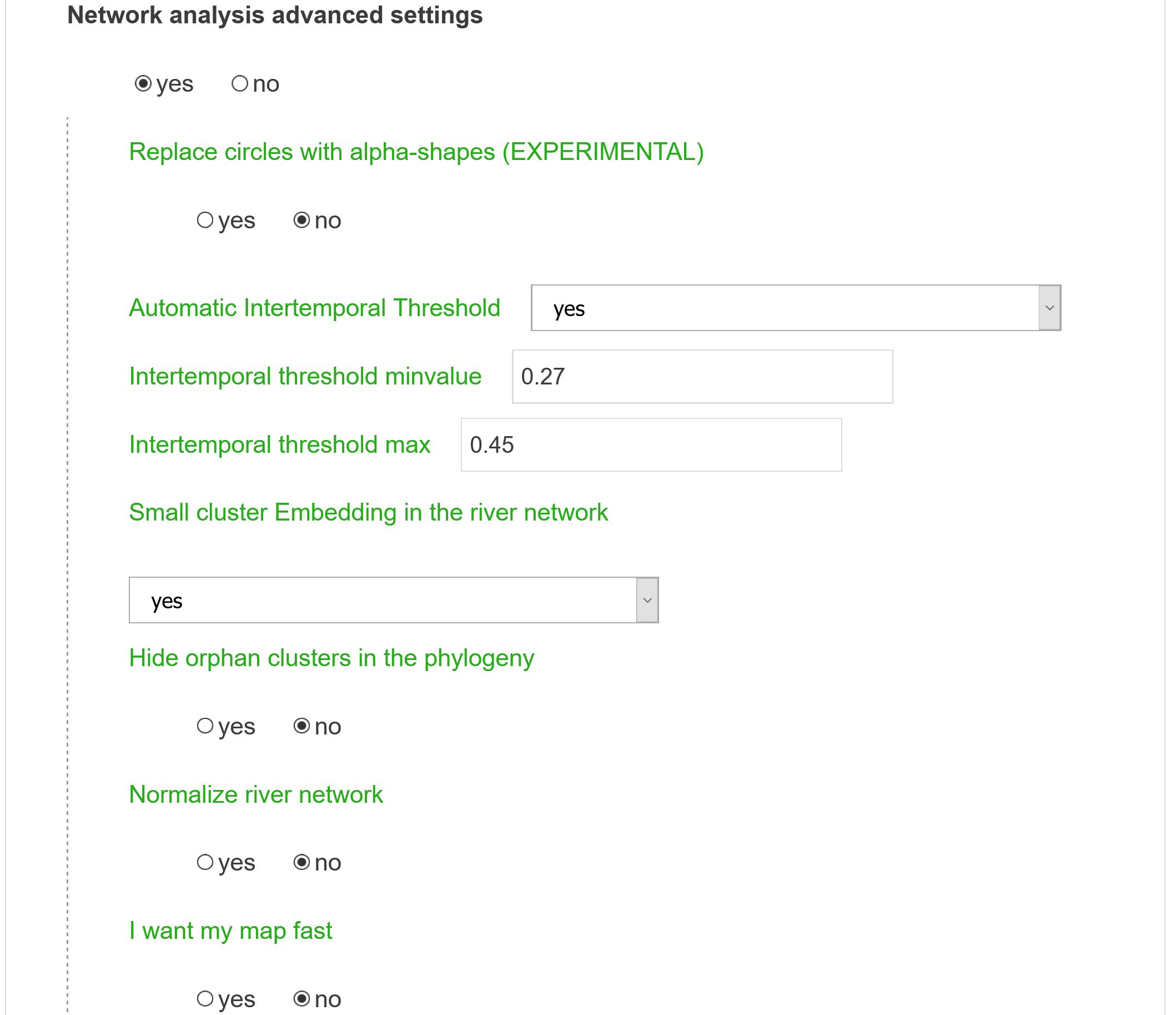
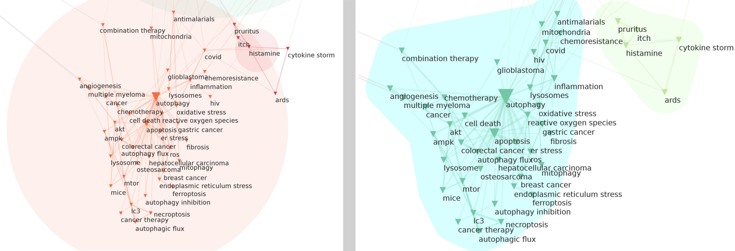
Replace circles with alpha-shapes

This option changes the final layout of the communities around nodes. Instead of circles whose sizes are proportional to the number of articles assigned to a given cluster (if Project records onto clusters option was activated), alpha-shapes are drawn for a more “organic” outcome.

Automatic Intertemporal Threshold

This refers to the threshold value used to create inter-temporal links when constructing river networks (tubes). This threshold is computed such that the total number of bifurcation in the final river network scales with the square root of the number of clusters overall (in all time ranges). Nevertheless one can manually tweak the parameter (Intertemporal threshold minvalue) to only consider stronger or weaker links connecting temporally successive clusters.

Intertemporal threshold minvalue

Only clusters intertemporally connected with a similarity above the threshold will be connected in the phylogeny a proximity above threshold will be conserved: should be between 0 (every possible links) and 1 (strictest option).

Intertemporal threshold max

If automatic intertemporal threshold is checked, final intertemporal threshold will not exceed this value.

Small cluster Embedding in the river network

A special procedure absorbs smaller clusters in the river network that may tend to stay isolated otherwise. This is not part of the original algorithm described in (Rule et al, 2015) but it still gives good empirical results.

Hide orphan clusters in the phylogeny

By default every cluster is shown, even isolated in the river network. If one changes this option to yes, only dynamically connected clusters will appear in the tube layout and disconnected clusters will be colored grey in every map.

Normalize river network

If yes, the size of clusters will be normalize at each time period.

I want my map fast

De-activate this option if experiencing memory errors or working with a very large corpus.

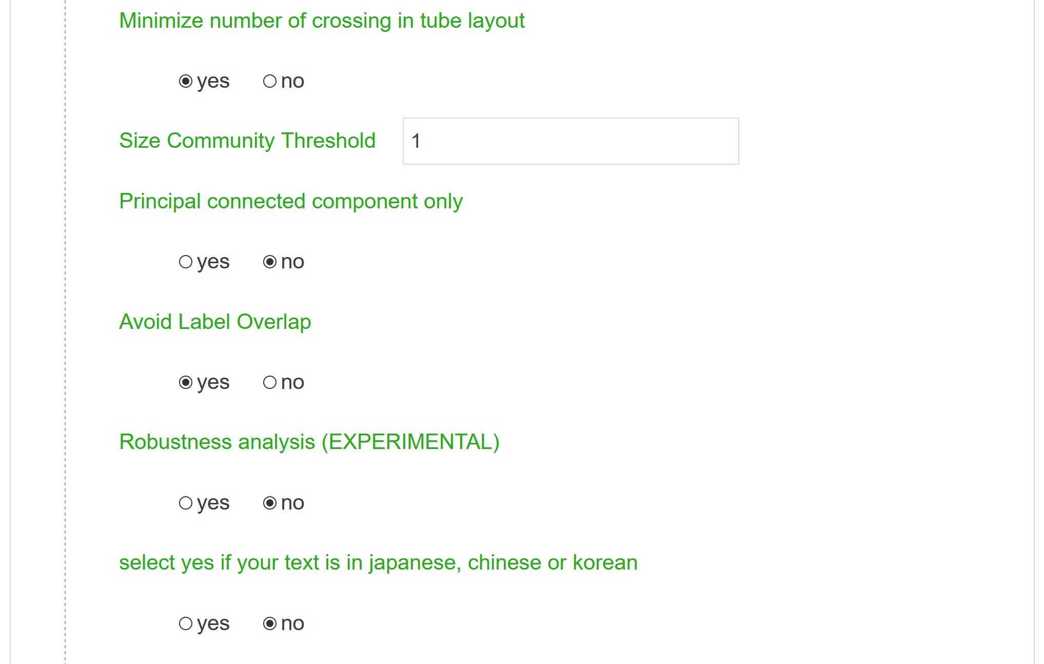
Minimize number of crossings in tube layout

If your river network is very large, minimizing the number of crossings may be very long. This option allows the user to accelerate the computation time (at the cost of a possibly less compelling visual outcome of the river network).

Size community Threshold

Only clusters whose size are above N will be considered: useful to get rid of “noisy” clusters made up of only two or three nodes.

Principal connected component only

Nodes that do not belong to the principal connected component will not be shown (they will be considered as isolated nodes).

Avoid label overlap

Original network Spatialization will be slightly modified to make the labels more readable.

Robustness analysis

Uncertain edges will be represented by dots. If activated, the final map is compared with the same map computed with the same parameters but on a random sample made of half of the original database. If edges are found in both map lines connecting nodes will stay solid, otherwise they will be dotted.

Select if…

If your text is in Japanese, Chinese or Korean, select this option

Remove nodes from the map

To highlight certain nodes and their labels, you can add a blank list of node labels: they will not appear in maps.

selectively remove certain node labels from the pdf map

Selectively remove certain node labels from the map from a uploaded resource list.

References

Aynaud, T. (2020). Python-louvain, Louvain algorithm for community detection. https://github.com/taynaud/python-louvain

Blondel, V. D., Guillaume, J.-L., Lambiotte, R., & Lefebvre, E. (2008). Fast unfolding of communities in large networks. J. Stat. Mech, 10008.

Lambiotte, R., Delvenne J.C., Barahona M. (2008). Laplacian dynamics and multiscale modular structure in networks – arXiv preprint arXiv:0812.1770

Fruchterman, T. M. J., & Reingold, E. M. (1991). Graph Drawing by Force-Directed Placement. Software: Practice and Experience, 21(11).

Martin Rosvall, & Bergstrom, C. T. (2008). Maps of random walks on complex networks reveal community structure. Proceedings of the National Academy of Sciences of the United States of America, 105(4), 1118–1123.

Palla, G., Derenyi, I., Farkas, I. J., & Vicsek, T. A. (2005). Uncovering the overlapping community structure of complex networks in nature and society. Nature, 435, 814.

Rule, A., Cointet, J. P., & Bearman, P. S. (2015). Lexical shifts, substantive changes, and continuity in State of the Union discourse, 1790–2014. Proceedings of the National Academy of Sciences, 112(35), 10837-10844.