The profiling script offers very similar analytical capacities than  contingency analysis.  Given two fields of interest, it will consider a target entity in the first field and produce a visualization of how biased the entities of the second field are distributed in documents which have been tagged by this target entity.

For instance, one may be interested to visualize the full profile of one source with respect to the year of publication, words being used in its documents or any kind of  metadata attached to individual documents.

Profiling visualisations

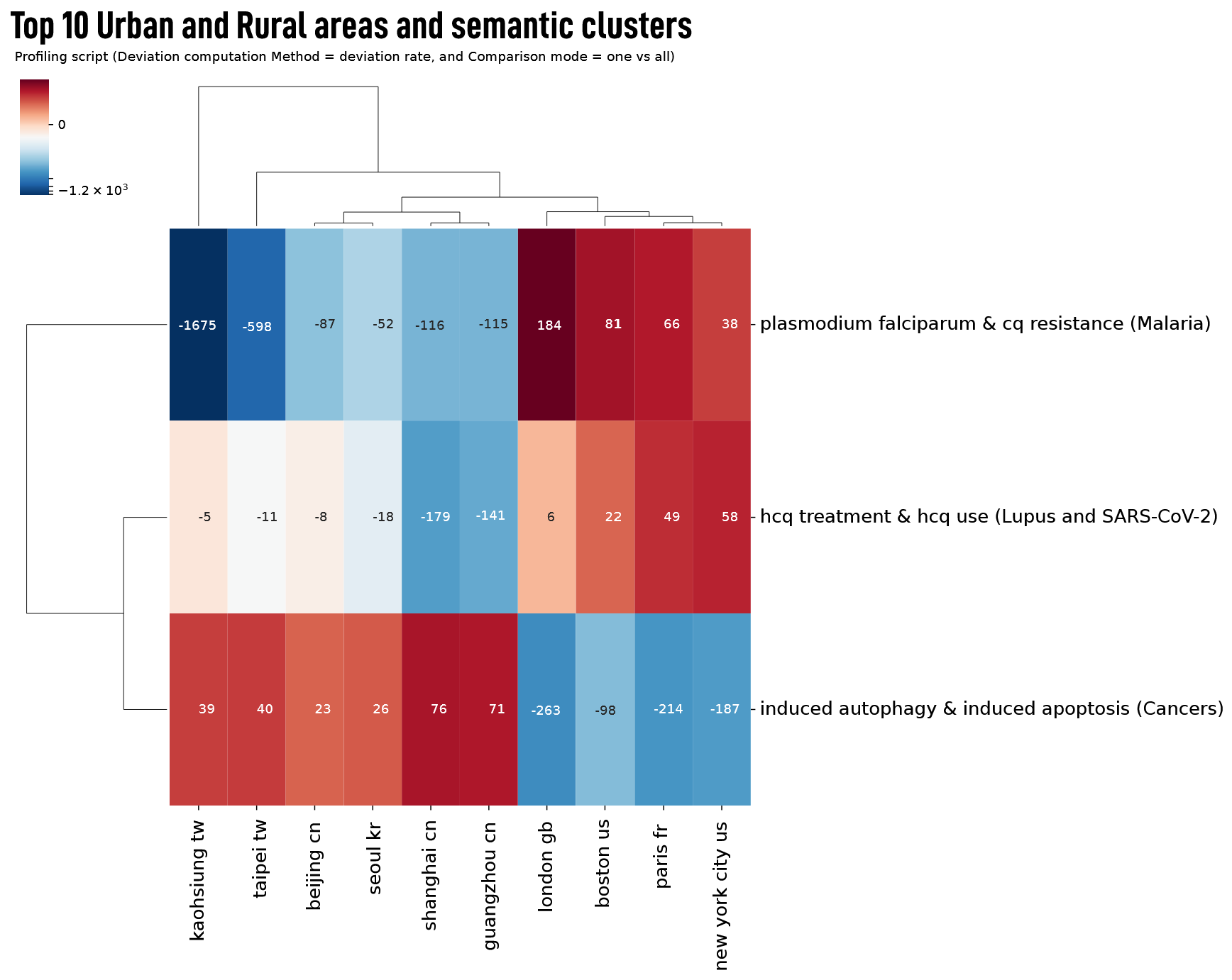
The first result shown is a matrix, in which the two selected variables are plotted. The dendrogram shows how close the intersection of the two variables is, or is not, from others combinations. In the example below, the first axis shows three semantic clusters (obtained after lexical extraction and network mapping scripts) and the second axis a list of the top 10 urban and rural areas (obtained after having geocoded the authors’ addresses and a spatial exploration script).

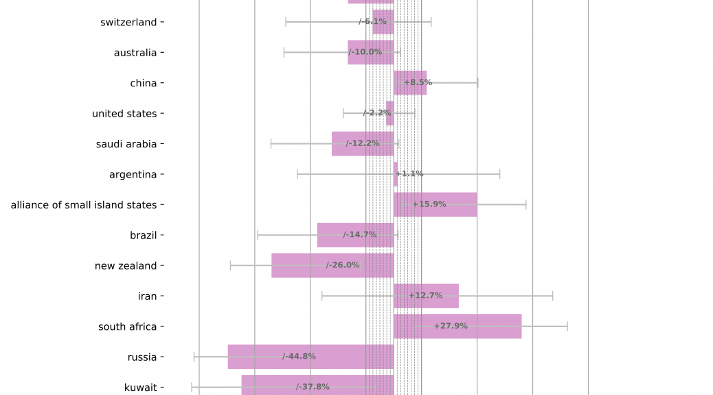
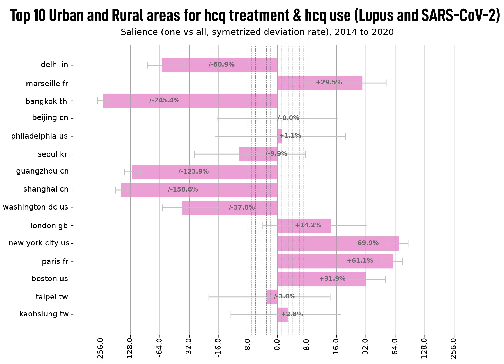
For further interpretation, a set of n histograms is produced, where n corresponds to the number of classes selected from the first field (see the example below where the histogram shown all the values of the top 10 urban and rural areas for the semantic clusters Lupus and SARS-Cov-2).

Profiling parameters

Nodes selection

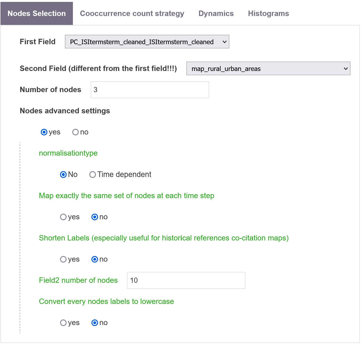
First Field

Define the first field from which nodes of your network will be selected. It is plotted as the Y axe in the matrix and its selected categories are used to compare the profiles of the second fields for the histograms.

Second Field

Define the second field from which nodes of your network will be selected, and must be different from the first field! It is plotted as X axe in the matrix, and all the selected categories are plotted in each histogram produced using the First Field.

Cooccurrence strategy

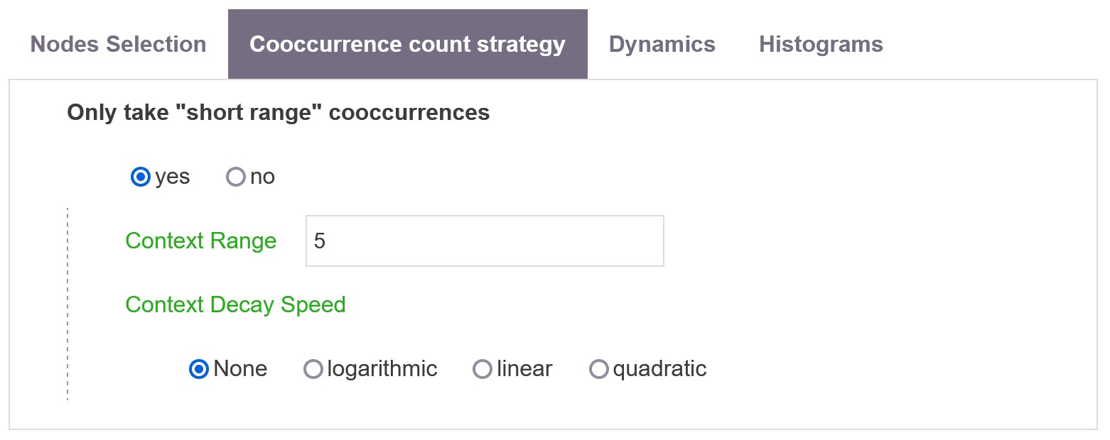
Only take “short range” cooccurrences

If yes, defines a maximal distance between two cooccurring items (e.g. sentences).

Context Range

Define the maximal distance (in number of sentences) between two terms for a cooccurrence to be valid (by default 5 sentences).

Context Decay Speed

You can also choose the speed at which cooccurrences strenght decay with the distance: None, Logarithmic, linear or quadratic.

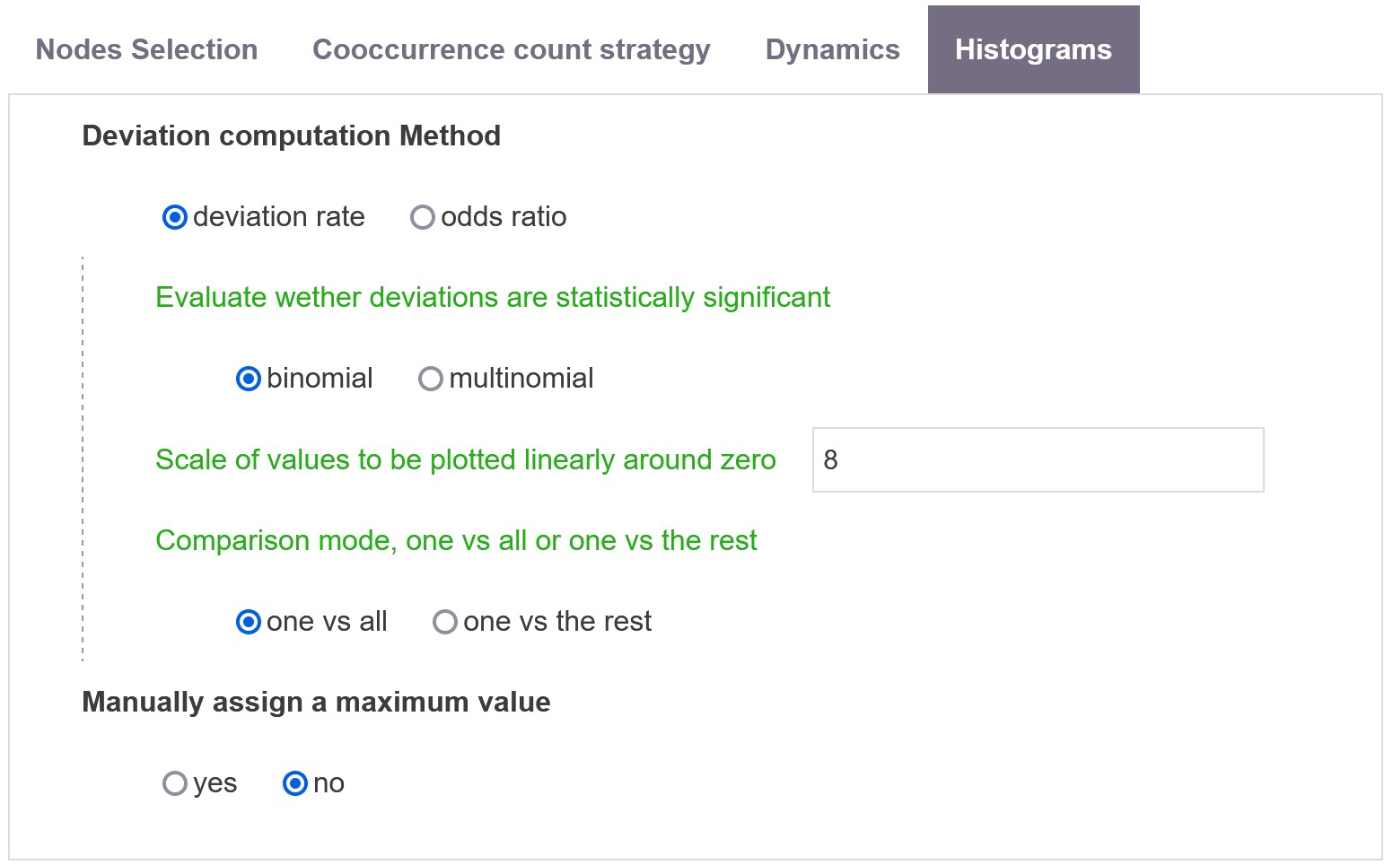
Histograms parameters

Two measures are possible for measuring the salience of entity i (from field 1) toward j (from field 2) .

Let’s consider a simple case that consists in measuring which delegation – among all the countries participating the Conference of the Parties – has been mentioning issues related to adaptation (identified thanks to a previous topic modeling) in the ENB corpus. Of course, we know that certain countries are more vocal than others. So we want our measure to be normalized, meaning that we will actually evaluate whether the proportion of times Tuvalu is talking about adaptation (compared to any other topic) is higher or smaller than the average value for all the countries .

Deviation rate

This deviation is simply measure as follows.

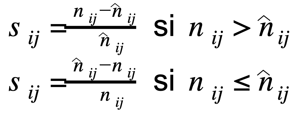We compare the empirical proportion of mentions of topic j by country i with its expected value that is the product of the proportions of times i is mentioned  by the raw number of times topic j is mentioned. We then measure a deviation rate that is symmetric, meaning that values can range from minus infinity to plus infinity.

Comparison mode, one vs all or one vs the rest

Chose the way one entity is compared to the rest: one versus all option (including Tuvalu) or one versus the rest option (excluding Tuvalu).

Evaluate whether deviations are statistically significant

Fisher exact test is performed on each cell of the matrix to measure the CI around the value of each score. Alternatively the CIs for the global multinomial distribution can be computed.

Scale of values to be plotted linearly around zero

Scale of values to be plotted linearly around zero, please enter an integer value (it corresponds to percentage points of deviation).

Odds ratio

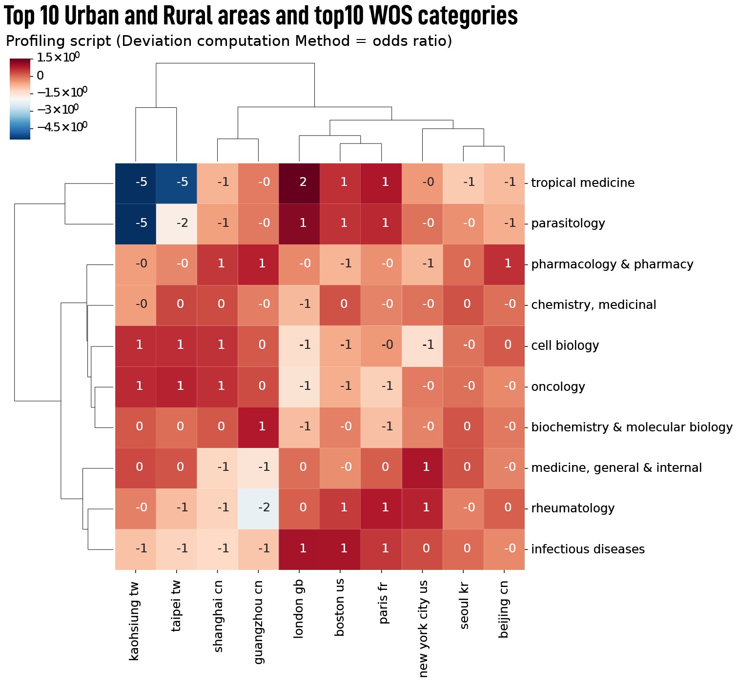The odds ratio is defined as the ratio between the probability of an event (such as an disease) occurring in group A and the probability of the same event occurring in group B. In the same way as for a racehorse: a horse at 3 to 1, has a 1-in-4 chance of winning.

As for the deviation rate, it has been symmetrized, meaning:

• >0: the frequency of the event (e.g. tropical medicine) is more frequent for a category (e.g. London gd), than for the rest of the corpus.
• =0: the event is equally frequent in both groups (e.g. medicine, general & internal for Paris fr, is equal to the distribution of this topic in the rest of the corpus).
• <0: the frequency of the event (e.g. tropical medicine) is less frequent for a category (e.g. Tapei tw), than for the rest of the corpus;