This page describes the parameters regarding the edges of the maps in the mapping script.

 

Proximity measure

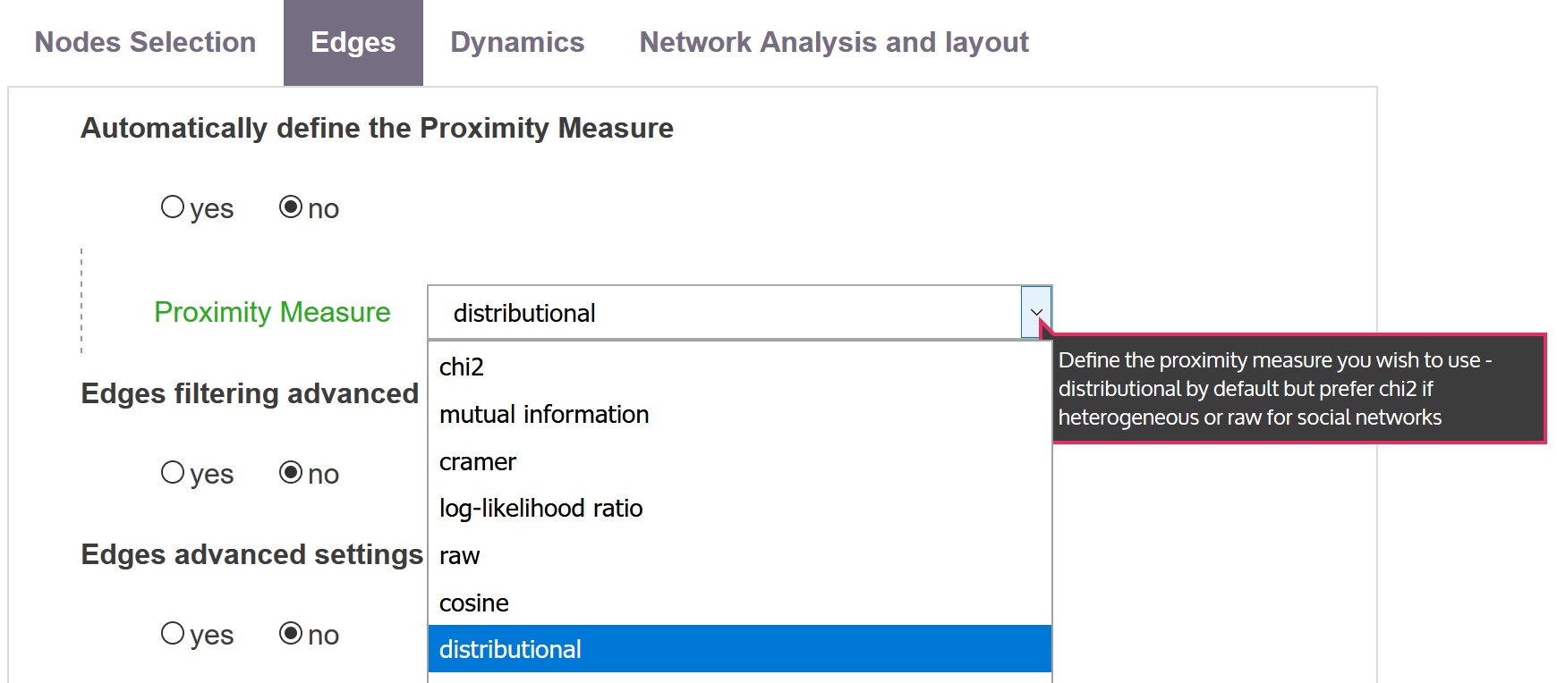
Proximity Measure

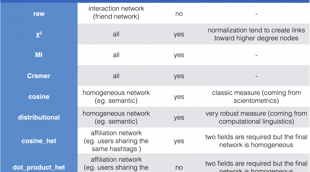
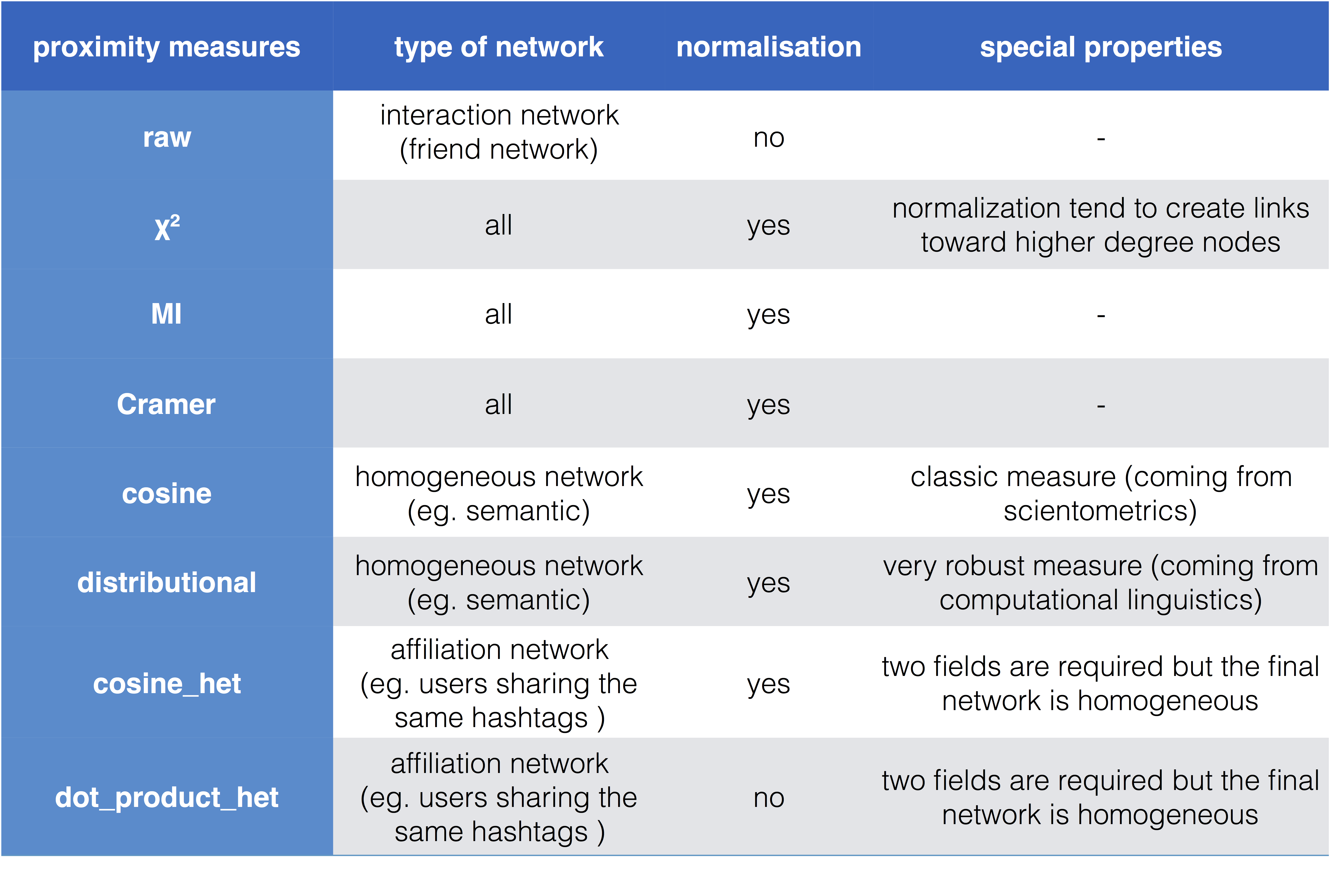
Once you have defined the fields of inquiry along with the correct time periods, co-occurrence networks should be transformed according to a given proximity measure. One can choose co-occurrences based direct (chi2, mutual information, raw, cramer) or indirect measures (cosine, distributional). Direct measures only take into account the raw co-occurrence number between two nodes while indirect measures account for the global distribution of co-occurrences of the two target nodes with all the other nodes.

Usually a standard strategy is to choose direct measures like chi2 for heterogeneous network  and indirect measure like distributional measure (or cosine more classically)  for homogeneous networks. This is the default behavior of the script if you don’t specify any metrics at this step.

Raw measure is also useful when one does not want to affect the original co-occurrences statistics, for example when plotting a collaboration network.

Heterogeneous measures (with the “het” suffix) allow the production of affiliation networks made of nodes from the first field only, whose proximity is computed by comparing their profile according to the second field. The scalar product or the cosine measure is then used to provide networks such as authors connected when sharing the same research interests.

A more thorough and technical explanation of the metrics are available on the metrics page.

Network Filtering: edges filtering advanced settings

An important step when producing a network map is to carefully define the filtering steps. Edges of the weighted network (the weight being equal to proximities between nodes) should be filtered in order to get rid of insignificant edges that may make it difficult for users to visualize its most significant features. Three possibilities are offered: (i) exclude any link whose weight is below the distance threshold, (ii) only select the N most significant edges (top edges according to their weight), (iii) only select the N edges connected to the closest neighbours of each node in the network (top neighbours).

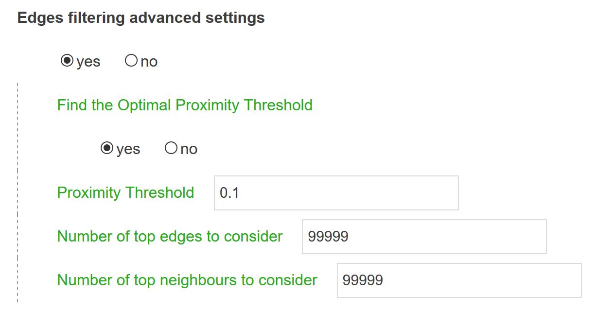
Find the Optimal Proximity Threshold

With Find the Optimal Proximity Threshold on yes (default value) CorText Manager uses a strategy to determine automatically for users a threshold where: just before, the network is divided in subcomponents (unliked partitions of the graph) and, just after, nodes of network are more widely linked to the other nodes. So, this strategy tends to minimize the number of links while conserving the overall connectiveness of the network. This process is a heuristic discussed in Jean-Philippe Cointet’s HDR, which comes from earlier work on tipping and contagion mechanisms in networks. “We therefore need to find a compromise between the presence of connections between clusters, so as to be able to situate them relatively to each other in the global space, and a maximum draining of the network’s links to reveal the boundaries of the clusters as best we can. To achieve this trade-off, an effective strategy is simply to find for our similarity network the critical threshold at which it makes its phase transition, i.e. the precise threshold at which the main connected component that makes it up disintegrates into several disconnected continents. In practice, we don’t stop at the first node that breaks off, but at the first cluster of nodes that breaks off (as, it would be enough for an exotic term in the context of the corpus to have slipped into the list of entities to be mapped to lower the threshold dangerously). By defining a similarity threshold slightly lower than this critical one, we generally obtain a network whose clusters are well structured but still connected to each other, allowing us to propose a global interpretation” (Jean-Philippe Cointet, 2017, p107).

Proximity Threshold

If users want to change this behaviour, choose no for Find the Optimal Proximity Threshold, and change the Proximity Threshold parameter. One should also keep in mind that direct measure cannot be below 0 but have no upper values (except for cramer distance always below 1) and that indirect proximity measures are comprised between 0 and 1.

Number of top neighbours to consider

Although users are free to define their own strategy when filtering, a simple rule of thumb is to focus on top neighbours filtering with indirect measures and distance threshold or top edges filtering with direct measures. In an adjacent matrix based on a RAW frequency, a top 3 neighbours of a given node A, means that are selected only the 3 highest values for the nodes of the networks linked to the node A (e.g. nodes B, C, D). But nodes A can be in the top 3 neighbours list of other nodes of the network (e.g. nodes E and F), so have in total more than 3 edges. In this example, E and F nodes are not in the top 3 edges list of A, but A is in the top 3 edges list of E and F… Selecting the Number of top neighbours to consider, is a strategy that keep what matters locally for each node, by preserving a certain degree of the overall network structure (useful, for example, to directly catch how intense are the relations in a coauthorship network or in a collaboration network between metropolitan areas…).

Edges advanced settings

The heterogeneous edges advanced option allows, when two different fields have been selected, to compute not only links between nodes in each field but also links between nodes falling in the same category.

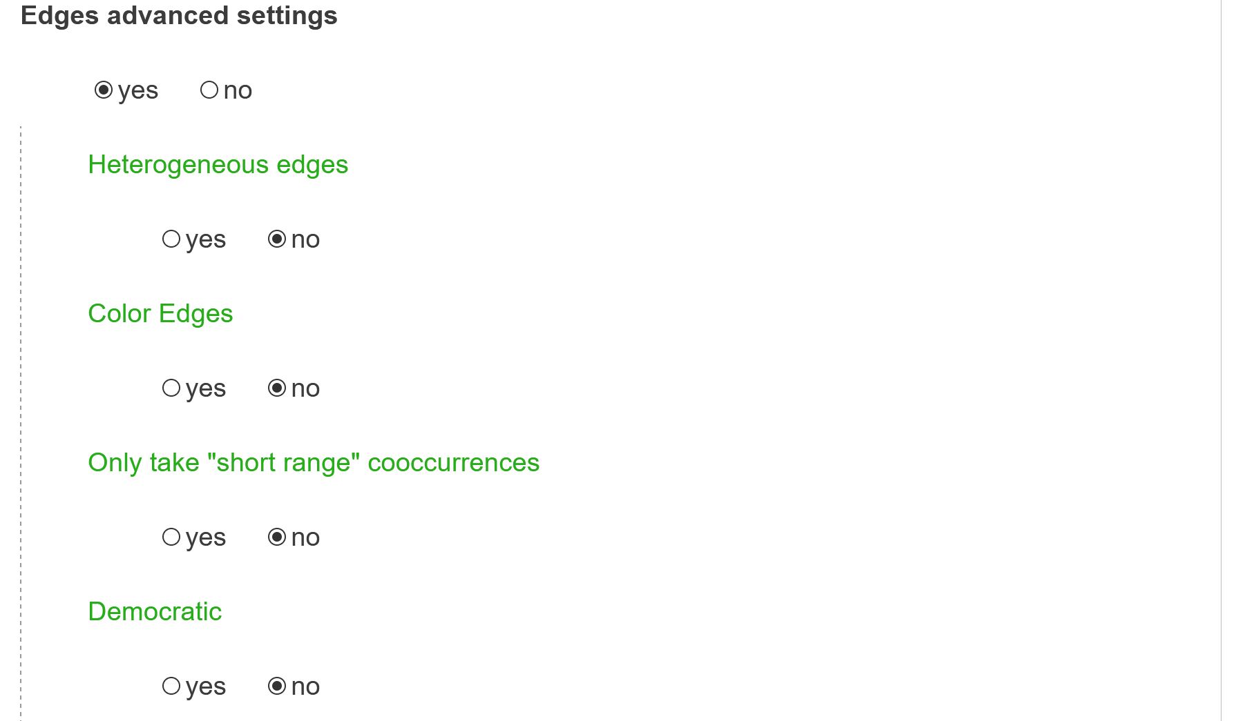
Heterogeneous edges

If your network is heterogeneous, do you want to consider every types of edges (choice: yes) or only edges connecting field 1 nodes to field 2 nodes (choice: no).

Color Edges

Edges will be colored according to the color of the node.

Only take “short range” co-occurences

This parameter allows you to control the range over which a co-occurrence is valid. It is especially useful when producing semantic maps of long documents. By default every joint appearance of two words in a record shall be considered as a co-occurrent event even if the two words are very far apart. If one activates the short-range option, when it is possible to define the maximum number of separating sentences between two words should be used to  consider the cooccurrences event to be significant. Classically, 5 to 10 sentences seems a reasonable value. Additionally, use the context decay speed, if you wish to weight the effect of co-occurence by a factor inversely proportional to the distance (still in number of sentences) between two words.

Democratic

This last option is still experimental. By default, for each document, a group is built connecting every pair of entities. For instance, author co-occurrence matrix will index collaboration between each pair of co-authors. It seems a reasonable assumption, but one may be tempted not to give too much importance to very large events gathering dozens or even hundreds of authors compared to smaller events. Put differently, by default, two people collaborating in a very large team have the same weight in the final map than two people working on their own. This option alleviates this effect and guarantees that each article have the same contribution to the final map.

References

Jean-Philippe Cointet. La cartographie des traces textuelles comme méthodologie d’enquête en sciences sociales. Sociologie. École normale supérieure, 2017. ⟨tel-03626011⟩