Geographical phenomena are by nature distributed. To deliver geographical coordinate to an address is one thing, but for the purpose of spatial analysis it is often necessary to aggregate geographical information, and associated data, on a more suitable scale. It is the case, for example, for analysing inter-urban or regional spatial dynamics based on human activities.

This aggregation, in a given area, of geographical points of different nature (organization name, building name, street number, city name …) located at different scales (points or centroids) is called a geospatial join. It consists for each point (couple of coordinates) to identify the shape (as a city or a region: multiple points with coordinates linked by lines) to which it belongs. Once this shape is identified, and all the points listed, it is possible: 1- to calculate and visualize the distribution of the phenomenon across these areas, 2- as well as to associate other variables already stored in your datasets (thematic clusters, keywords …).

A common question raised by this operation, is the choice of relevant boundaries. In many studies the national administrative boundaries are chosen. These approaches face two major issues:

• Inconstancies when comparing two countries, as their intranational boundaries may have been built for specific organizational purposes (with a large variety of sizes) and administrative needs (number of administrative scales);
• Regional boundaries may hide strong spatial and social discontinuities, such as between a predominant urban area and a wide area dedicated to agriculture within the same entity.

To answer these two classes of problems, several remarkable attempts exist. The NUTS (EUROSTAT, 2008) has enabled intercountry comparisons in Europe, by harmonizing population per shape. With the Functional Urban Areas (Brezzi, 2012; OECD, 2012) OECD proposes to identify urban areas based on a core dense space (inhabitants’ density) with in addition areas that functionally depend on it (using commuting data). Other initiatives are moving away from administrative boundaries to rely only on the internal dynamics of the data studied by proposing, for example, endogenous geographical clusters. This enables both to have a global coverage and to no longer suffer to socio-spatial discontinuities as, in these cases, only the spatial concentration of the phenomena studied matters. Applied to the world science production, 80% of the activities is located in less than 500 urban areas. NETSCITY enable to locate bibliographic records of scientific articles within these areas, where close cities have been clustered (Maisonobe, Jégou, & Eckert, 2018; Maisonobe, Jégou, Yakimovich, & Cabanac, 2019). In a more disaggregated manner: addresses are widely distributed across geographical space. Using a density-based algorithm helps to identify areas where the activities are concentrated (Villard & Laredo, 2016; Villard & Revollo, 2015).

The CorText Geospatial Exploration Tool offers an original way to solve this, by combining in one unique tool a large variety of well-established sources of shapes. The present service proposes basemaps at four different scales:

• URA boundaries: for Urban and Rural Areas, which includes a worldwide coverage of urban areas and, in the meantime, regionalized boundaries (states, departments, provinces, prefectures…) of the areas which are outside of the highest concentrations of inhabitants;
• UA boundaries: for Urban Area, is a subset extracted from the previous geographical layer, which includes only urban areas, to make it simpler (if needed);
• Regional boundaries: a worldwide layer for regional analysis;
• Country boundaries.

Geospatial Exploration CorText Tool is designed to work after CorText Geocoding script as it needs coordinates (longitude, latitude) in a specific format (e.g. 104.068108|30.652751 for longitude|latitude).

Building the urban areas

The urban areas have been built based on several sources of information:

• 667 Functional Urban Areas in Europe (EU-28): built following the core analysis by density and with the addition of dependant areas (Lavalle, Kompil, & Aurambout, 2015);
• 17 Urban Areas for European associated countries: Urban Audit 2011-2014 (European Commission Eurostat, 2015);
• 104 Functional Urban Areas: from OECD, for Mexico, Colombia, South Korea, Japan, Chili, Canada, Australia (Brezzi, 2012; OECD, 2012);
• 450 Urban areas in US: US Census Bureau, Cartographic Boundary of Urban Areas, 2017 (United States Census Bureau – Geography Program, 2017);
• 375 Chinese Urban Areas: from Beijing City Lab, from an analysis of population density (based on BCL Data 19) in 2012 (Long & Shen, 2016);
• 2,587 Urban Areas for the rest of the world: Natural Earth, “derived from MODIS satellite data at 1 km resolution”, based on a method to capture dense light areas on earth (Patterson & Vaughn Kelso, 2014; Schneider, Friedl, & Woodcock, 2003).

These 4,200 urban areas have been combined in one layer (see “modifications made on URA” section to know how they have been cleaned).

Be aware that inter-sources comparisons might suffer of a lack of consistency. As different methods have been used to produce the different types of urban areas, the average surface vary (e.g. between functional urban areas and urban areas from dense light zones). Nevertheless, this is a useful and original way to aggregate locations (addresses, cities…) that are next to a core dense urban center, and to reduce drastically the geographical spread of the data with a worldwide approach.

Adding rural areas

To conduce analyses outside urban areas, we have added a regional layer published by Natural Earth (Patterson & Vaughn Kelso, 2014). This layer gathers “first-order administrative boundaries and polygons for all but a few tiny countries. It includes name attributes (including diacritical marks), name variants, and some statistical codes (FIPS, ISO, HASC)”. It corresponds to the country regional scale (state, province, prefecture, department…).
These new entities have been built to fill portions of geographical space which are outside urban areas. Consequently, urban areas can overlap two or more original administrative boundaries from the regional shapes, and they can cross countries borders. Regional shapes can completely disappear in favor of the corresponding urban areas, when they are wider.

In total 4,428 rural areas have been added.

Urban and Rural Areas (URA) classes

Following the classification proposed by OECD for FUA, urban areas are classified based on their population. In order to apply this classification to all the areas, whatever they are rural or urban, 349,202 cities from GeoNames (GeoNames, 2018) with at least 10 inhabitants have been studied. Estimated population is summed across the urban or rural areas: 80% of the number of inhabitants has been added to GeoNames between 2012 and 2015 (and the first entry is from 2006). Based on this estimation, we have finally kept only urban areas with more than 50,000 inhabitants. A new class for rural areas below this threshold has been added. Our full classification is the following:

• Very small rural areas (rural areas below 50,000. All urban areas with a population below 50,000 have been withdrawn);
• Small (urban or rural) with population between 50,000 and 100,000;
• Medium-sized (urban or rural) areas: with population between 100,000 and 250,000;
• Metropolitan or rural areas: with population between 250,000 and 1.5 million;
• Large (rural or metropolitan) areas: with population above 1.5 million.

Toponym names from GeoNames have been used to name urban areas, by selecting the English name of most populated place in the area. The names of the rural areas remain the names provided by the original sources.

A suffix ” – rural” is added to the label name for rural areas which have a portion of their territories covers by an urban area (e.g. Gard – rural). At the opposite, a rural area without the suffix corresponds exactly to the shape in the original source (e.g. Aveyron).

Modifications made on URA and added variables

When merging several geographical sources of information, numerous problems might occur. Many modifications have been made to improve the overall quality of the URA layer:

• Overlapping areas: updates made on the shared boundary between Annecy and Geneva. Ceuta and Nador (Nador / Melilla) were belonging both to Morocco and Spain; Sinuiju (North Korea) and Dandong (China) were partially overlapping; Yuen Long Kau in Hong Kong peninsula were overlapping;
• Merged urban areas: Hong Kong (island) and Kowloon (continental part, also named Tsuen Wan) have been merged while Yuen Long Kau stayed separated. Guangzhou (Shenzhen-Guangzhou conurbation) and Yuen Long Kau in the Hong Kong peninsula have been separated;
• Changes due to the hydrography: River Thames is not any more excluded from the London urban area, many lackes (and some forests) have been removed to Chinese and Russian urban areas;
• Many other changes (manly merges and boundaries updates) have been made, ask us to have the full list. You may also find new ones, please contact us.

Whatever the layer is, some extra variables have been calculated in order to enable further works. These variables might be also useful to link areas to the original data source. Here is the list that all the layers share: name of the areas, name of the source, ID in the source, centroid of the shape to enable further network calculations (longitude and latitude of the centroid), estimated population which is used for density calculation into the maps (see above for the method used with GeoNames), surface of the areas in square kilometres (used for the density calculation into the maps).

GeoSpatial join parameters

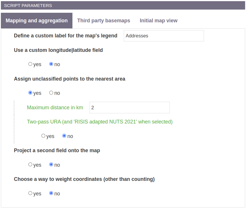
Use a custom longitude|latitude field

The first step is to select which field contains the geographical coordinates (Use a custom longitude|latitude field). This field is produced by CorText Geocoding service as geo_longitude_latitude which is selected by default.

If you want to use your own list of longitude/latitude coordinates, you can upload a csv file where a column holds the two values separated by a pipe (e.g. 104.068108|30.652751). If you have multiple values per document, you may use a separator (e.g. 104.068108|30.652751***4.89973|52.37243 in a cell). In that case, select yes and precise the name of the field.

CorText GeoSpatial Exploration tool uses shapes with a high level of precision: from 10 meters to 5 kilometers depending the layer and the source. For geographical space: distance matters! So, on one hand, at this level of precision a geocoded address may not fall into the shape for a small distance (as for an address in a park, next to a river or in a port, in an island… excluded from the urban areas). On the other hand, an address which is close to a boarder, may fall outside the right shape for only a few meters due to some simplification of the boundaries.

Assign unclassified points to the nearest area

If you want to avoid these situations, you may choose the parameter Assign unclassified points to the nearest area. If yes (which is the default behaviour), CorText Manager will look for each outlier point (geocoded address), in a given perimeter (by default 2 km), which are the closest centroids of shapes (urban or rural areas, regions…). After having selected the three closest centroids, CorText Manager will identify for the outlier which is the closest boundary between the three shapes selected by their centroids. Finally, the point will be affected to this area.

Two-pass URA

By default the outlier points will be attributed to the nearest area found, whatever if it is a urban area or a rural area. When Two-pass URA is selected as Yes, the spatial join will proceed first with urban areas only, and finds the nearest points (geocoded) in a given perimeter (set with the Maximum distance in km parameter), and secondly with rural areas for the remaining points. This parameter creates a buffer zone around the urban areas of a specific distance (2 km if using the default value). It aggregates locations (geocoded addresses) with the urban areas if they are close to it, even if they would have fall in a rural area. This strategy is applied to the Urban and Rural Areas layer, and to RISIS adapated NUTS when selected in the third party basemaps list.

Thus, for ‘RISIS adapted NUTS 2021’ (Two-pass URA is selected as Yes and ‘RISIS adapted NUTS 2021’ is selected in the Third party basemaps tab), longitude and latitude coordinates are processed as follows:

• the spatial join proceeds first with `Knowledge hubs` + `Metropolitan regions` and finds the nearest points within the defined perimeter (2 km by default);
• and then includes all the other classes of NUTS (adapted NUTS2, Original NUTS 2, Original NUTS3) for the remaining coordinates, using also the buffer zone strategy.

Project a second variable onto the map

If Project a second variable onto the map is selected, a given field is used to tag the shapes with the Top N elements. It could be useful for semantic clusters, or to draw profiles with classes for regions or urban and rural areas. This parameter enriches the legend of a map with this Top N elements and produces a csv file for each layer.

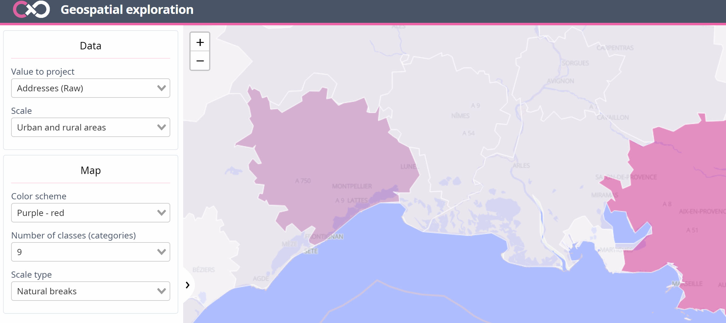
Interactions with the choropleth maps

Several interactions are accessible to explore the data in different ways.

Classifying URA

Two methods are accessible to classify the values projected onto the maps :

Quantiles

The effectif of shapes represented on the map is divided in N classes. Each class receives the same amount of shapes;

Natural break

Jenks natural breaks optimization (Jenks, 1977) is made to classify data for choropleth map in a more human readable way. It tends to “minimize each class’s average deviation from the class mean, while maximizing each class’s deviation from the means of the other” classes. We are using here a recent optimization (Schnurr, 2016) of the orginal method.

Precision of the shapes

Due to the precision of the layers, it would have been too heavy to load it into a browser. The full layers are used for the geospatial join (to ensure the highest possible accuracy), but the shapes visualized onto maps have been widely simplified. We have used the Douglas-peucker algorithm (Douglas Thomas K., 1973) to reduce the number of points of the shapes’ boundaries. Up to 90% of the points (in some portions of the URA layer) have been removed and replaced by lines, with two constraints that the algorithm should follow:

• none of the shapes should completely disappear (so, the minimal shape is a triangle);
• take in account shared lines (e.g. boundaries between two countries, to avoid holes between them).

Export the map

You may want to do further work with the maps outside CorText Manager: you can export the maps in geojson format. Keep in mind the layers and shapes you will download are the one which have been simplified. Furthermore, only shapes with a value are mapped. So,built you will gather and download in the exported geojson file only shapes where at least one point from your dataset have been projected. Please ask us if you want the precise version of URA layer with all shapes.

Third party basemaps

Following the same methodological steps and parameters, you can add one extra basemap.

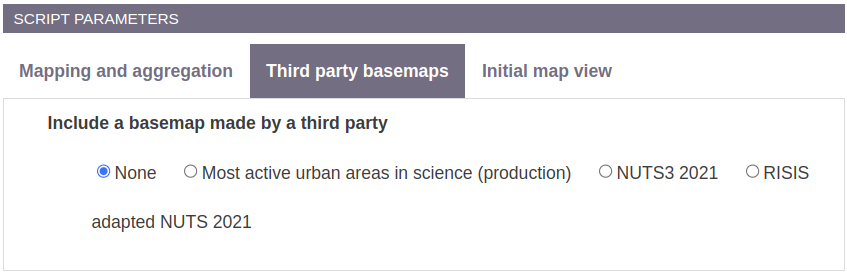
This added basemap may be particularly useful depending needs and data coverage.

Most active urban areas in science production

This open access dataset covers the places where 80% of the world’s science was produced (scientific publications listed in the Web of Science) between 1999 and 2014 (Maisonobe, Jégou, & Eckert, 2018). This basemap fuel the NETSCITY web application where it is possible to analyze scientific datasets with these 480 geographical clusters and to export maps or statistics.

NUTS3

For Nomenclature of Territorial Units for Statistics (EUROSTAT, 2008) covers european member states and associated countries. It has been built to produce statistics in Europe at country subdivisions scale. CorText Manager uses NUTS3 2021 basemap, which gathers administrative entities with a population in average between 150,000 and 800,000. It has been published in 2021 (© EuroGeographics for the administrative boundaries).

RISIS adapted NUTS 2021

Adapted NUTS have been produced as part of the H2020 RISIS project. Compared with NUTS3, it focuses on large agglomerations, while remaining fully compatible with the EUROSTAT NUTS regional classification. This compatibility allows combining data with regional statistics (at NUTS3 level, 2021 edition) from EUROSTAT. “More precisely, the classification includes EUROSTAT metropolitan regions (based on the aggregation of NUTS3-level regions) and NUTS2 regions for the remaining areas; further, a few additional centers for knowledge production […] have been singled out at NUTS3 level. The resulting classification is therefore more fine-grained than NUTS2 in the areas with sizeable knowledge production, but at the same time recognizes the central role of metropolitan areas in knowledge production.” (Lepori, B., & Guerini, M., 2020, https://zenodo.org/record/3752861).

Improvements and known issues

Solved issues

Known issues

Section to expand with your feedbacks.

Example of usage

This example uses a 3D printing dataset with all scientific publications published in a given time period.

1. Run Text > Lexical Extraction script on Abstract, ISIID, Keywords, Title fields with default parameters (see documentation page). Results are stored in Terms field;
2. Run Analysis > Network Mapping script with Terms as First Field and Second Field with default parameters in order to build semantic clusters (see documentation page). Results are stored in PC_Terms_Terms field;
3. Run Space > Geocoding script with default parameters (see documentation page), addresses of the authors are stored in Address field. The results of the script (longitude|latitude coordinates) are stored in geo_longitude_latitude field;
4. Run Space > Geospatial Exploration script with geo_longitude_latitude as the field which contains geographical coordinates, Assign unclassified points to the nearest area as Yes, Two-pass URA as Yes, and Project a second variable onto the map as Yes with PC_Terms_Terms to show in the maps the top 3 semantic clusters for each shapes;
5. When calculation has ended, in the results dashboard, click on the eye next to map.geocortext to open the web mapping tool;

And enjoy your maps !

URA data sources references

Pay attention that, depending on the section of the map studied, you will need to cite the related work. The source of the urban and rural areas, with their original IDs, is kept in the data provided by CorText Manager in order to make you able to cite them properly.

Brezzi, M. (2012). Redefining urban: a new way to measure metropolitan areas. OECD Publishing. Retrieved from http://www.oecdbookshop.org/browse.asp?pid=title-detail&lang=en&ds=&ISB=9789264174054

European Commission Eurostat. (2015). Urban Audit 2011–2014. Retrieved from https://ec.europa.eu/eurostat/web/gisco/geodata/reference-data/administrative-units-statistical-units/urban-audit#ua11-14

GeoNames. (2018). GeoNames, worldwide multilingual open data source on toponyms. Retrieved from www.geonames.org

Lavalle, C., Kompil, M., & Aurambout, J.-P. (2015). UI – Boundaries for the functional urban areas (LUISA Platform REF2014). Retrieved from http://data.europa.eu/89h/jrc-luisa-ui-boundaries-fua

Long, Y., & Shen, Y. (2016). Mapping parcel-level urban areas for a large geographical area. Annals of the American Association of Geographers, 106(1), 96–113. Retrieved from http://arxiv.org/abs/1403.5864%0Ahttp://www.arxiv.org/pdf/1403.5864.pdf

OECD. (2012). Redefining “Urban”: A New Way to Measure Metropolitan Areas. OECD Publishing, (September), 1–9. https://doi.org/10.1787/9789264174108-en

Patterson, T., & Vaughn Kelso, N. (2014). Natural Earth, 1–2. Retrieved from https://www.naturalearthdata.com/about/terms-of-use/

Schneider, A., Friedl, M., & Woodcock, C. E. (2003). Mapping Urban Areas by Fusing Multiple Sources of Coarse Resolution Remotely Sensed Data. Photogrammetric Engineering and Remote Sensing Remote Sensing, 69(C), 1377–1386.

United States Census Bureau – Geography Program. (2017). Urban areas. Retrieved August 22, 2019, from https://www.census.gov/programs-surveys/geography/geographies/mapping-files.2017.html

To add extra-variables in CorText Manager on top of the URA (see: corpus list indexer) or to explore the full list of URA, you may what to download the file below. It includes also, for each shape, the full list of references you should cite.

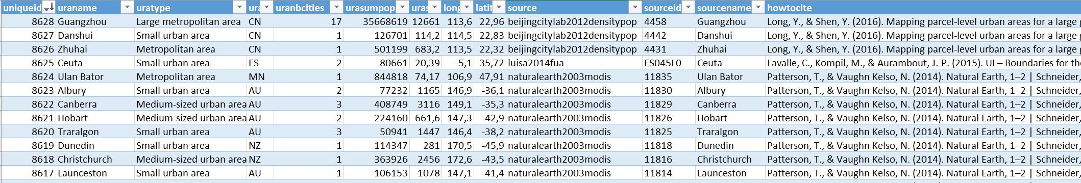
Download the full URA definition file

References

Douglas Thomas K., D. H. and P. (1973). Algorithms for the Reduction of the Number of Points Required to Represent a Digitized Line or Its Caricature. Canadian Cartographer, 10(2).

EUROSTAT. (2008). Nomenclature of Territorial Units for Statistics. Retrieved from http://epp.eurostat.ec.europa.eu/portal/page/portal/nuts_nomenclature/introduction

Jenks, G. F. (1977). Optimal data classification for choropleth maps. Occasional Paper No. 2, Dept. Geography, Univ. Kansas, 24.

Maisonobe, M., Jégou, L., & Eckert, D. (2018). Delineating urban agglomerations across the world: a dataset for studying the spatial distribution of academic research at city level. Cybergeo. https://doi.org/10.4000/cybergeo.29637

Maisonobe, M., Jégou, L., Yakimovich, N., & Cabanac, G. (2019). NETSCITY : a geospatial application to analyse and map world scale production and collaboration data between cities. In International Conference on Scientometrics and Informetrics.

Schnurr, D. (2016). Using clustering to create a new D3.js color scale. Medium. Retrieved from https://medium.com/@dschnr/using-clustering-to-create-a-new-d3-js-color-scale-dec4ccd639d2

Villard, L., & Laredo, P. (2016). Agglomeration and collaboration in knowledge absorptive capacities in emerging science and technologies: the case of nanosciences and technologies. In 3rd Geography of Innovation Conference. Toulouse.

Villard, L., & Revollo, M. (2015). GeoClust: a tool to study the geographical aggregation of activities. CorText. Retrieved from https://www.cortext.net/geoclust-a-tool-to-study-the-geographical-aggregation-of-activities/

Refer to this work

This set of methods have been funded by the European Union under Horizon2020 Research and Innovation Programme RISIS².

If you have found the tool and results useful, we would be grateful is you would refer to this work by citing it in your own documents or publications:

Villard, Lionel, Opsina, Juan Pablo & Medina, Luis Daniel (2019). CorText Geospatial Exploration Tool. ESIEE Paris, Paris Est University. https://docs.cortext.net/cortext-geospatial-exploration-tool/