How to use Terms Extraction

Textual fields definition

Select the textual fields you wish to analyze and index:

If one chooses to analyse a Web Of Science dataset, then the available textual fields would be Title, Abstract, Keywords (provided by authors), ISIID (Keywords provided by WOS) and Addresses.  

List length and terms list filtering

Lexical extraction script aims at identifying the most salient multi-terms according to statistical criteria (see technical description below). You can also exclude any term below a given minimum frequency. Another important parameter is the List length size you wish to extract. This parameter may have strong impact on script speed, so it is advised to keep this parameter below 1000.

language

Don’t forget to specify the language of your dataset – only french, german, spanish and english are taken into account. Spanish, German, Russian, Italian and Danish have been less extensively tested than French and English (any feedback is welcome!). If you select “Other”, no grammatical processing will be applied to the data, meaning only statistical criteria based on collocation of words will be used to derive phrases.

monograms

You are also given the possibility to exclude monograms (that is terms composed of only one word). It is advised to exclude monograms as they tend to be less informative terms.

Maximal length (max number of words)

It is also possible to limit the maximum number of words encapsulated in a multi-term. Three is reasonable, but feel free to try to identify longer multi-terms.

Optionally you can name the new indexation that will be generated

By default a new table Terms will be created. It is possible to choose a different name for this table and hence manage various indexes at the same time. The indexed variable will be suffixed by ISITerms + the string you entered. Please use simple characters (no accents, etc.) and avoid using spaces.

Advanced settings

These advanced options are described below.

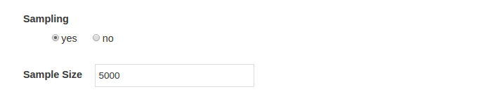
Sampling

For large datasets, and if you are advised to sample your original dataset. Terms extraction will only be based on sample sub-corpuses with a given number of documents (randomly drawn from original successive datasets). Nevertheless, detected terms will be indexed in the whole corpus whatever the sampling strategy.

Frequency (c-value) computation level

C-value calculation measure the unithood of multi-terms stem as proposed by Frantzi & Ananiadou (2000). The frequency of terms can be computed at the document level (meaning that terms frequency are computed based on the number of distinct documents they appear in) or at the sentence level (default choice, meaning that repetitions of a terms across sentences inside a document will be taken in account in the frequency calculation). As the frequencies of a term (main form) are calculated during the indexation process (so, after the extraction and selection of the relevant keywords), results for Frequency computation level are stored in the folder indexed_list, inside the multiterms_statistics_expanded.tsv file. See below the Example of lexical extraction.

Ranking Principle

The selection of most pertinent terms results from a trade-off between their specificity and their frequency (see technical explanations below). By default, specificity is computed as a chi2 score (summed over all words).t is also possible to use a simpler G2 (gf.idf for Global Frequency/Inverse Document Frequency derived from the well known TFIDF) score to do so. The G2 score is based on the assumption that interesting terms tend to be repeated within the same document. Another option is to use the “pigeonhole pertinence measure” which gives more weight to words which tend to cooccur several times per document (several pigeons in one pigeonhole). Pigeon score will identify words which occurrences tend to concentrate in a small set of documents (relatively to the term total frequency), pigeon score is equivalent to gf.idf but correcting for the over-representation of frequent words (as a consequence the measure is only valid for large enough documents, typically at least several sentences). One can also deactivate the role of specificity in the final ranking of extracted terms such that only top N most frequent terms will be retrieved (frequency). 

linguistic pre-processing

One can also totally deactivate the linguistic pre-processing (pos-tagging, chunking, stemming). It is useful when treating texts in other languages than English, French, German or Spanish, but also in cases where one does not want to reduce the extraction to a single grammatical class. 

grammatical criterion

By default, noun phrases are identified and extracted but you can also choose to try to identify adjectives or verbs.

Automatically index the corpus

The script first extracts a list of terms and then indexes the corpus (stored in the Terms field or a custom one). It is possible not to index the corpus by checking this box. If so, the standard field Terms won’t be erased (if one from a previous calculation already exits) or created (for a first attempt). It enables to generate a new list of terms, and to examine it in the tsv file, without replacing a previous indexed one.

Pivot Word

Only multi-terms containing this string will be extracted.

Starting Character

Only terms starting with this character shall be extracted. It comes in handy if you wish to index hashtags for instance (#). Simply deactivate linguistic pre-processing and make sure to also deactivate linguistic pre-processing in that case. 

Working with time series data

When having a time variable in your corpus, you may want to have a better view of the changes in term of vocabulary among time. It is particularly helpful to divide the lexical extraction in order to eventually follow radical changes of the vocabulary in your corpus produced over these periods.

In the Dynamics panel, one can temporally slice the corpus to apply different lexical extractions.

Number of time slices

Different lexical extraction process will be applied to the different time periods defined (either from the original time range or from a customized time range if one was computed before).

regular or homogeneous

Time slices are either regular, with a uniform distribution of timesteps per period, or homogeneous, with a uniform distribution of documents per period (same parameter than:  time slices distribution).

Methodological background

Automatic multi-terms extraction is a typical task in NLP, yet the existing tools are not always well suited when one wishes to extract only the most salient terms. As specificity computing is time and resource expansive, we have developed an automatic method to extract lists of terms that we suspect to be the best candidates for lexical extension. Thus we will be interested in groups of relevant terms featuring both high unithood (Frantzi, K. , Ananiadou S., & Mima H., 2000) and high termhood as defined in (Kageura, K., & Umino, B., 1996).

The whole processing of textual data can be described as follows: it first relies on classic linguistic processes that ends up defining sets of candidate noun phrases.

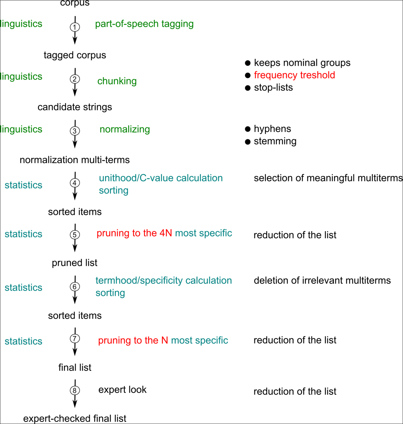
POS-tagging

Part-of-Speech Tagging tool first tags every terms according to its grammatical type : noun, adjective, verb, adverb, etc. CorTexT Manager uses Natural Language Toolkit (NLTK) for English and TreeTagger for the other languages (Helmut Schmid, 1994, 1995).

Chunking

Tags are then used to identify noun phrases in the corpus, a noun phrase can be minimally defined as a list of successive nouns and adjectives. This step builds the set of our possible multi-terms.

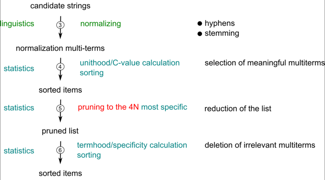
Normalizing

We correct small orthographical differences between multi-terms regarding the presence/absence of hyphens. For example: we consider that the multi-terms “single-strand polymer” and “single strand polymer” belong to the same class.

Stemming

Multi-terms can be gathered together if they share the same stem. For example, singular and plurals are automatically grouped into the same class (e.g. “fullerene” and “fullerenes” are two possible forms of the stem: “fullerene”). Porter’s stemmer is used for English (Porter, 1980),  when Snowball stemmers are used for French, German and Italian, both from NLTK. For the other languages (Da, Ru, Es, Other), a lemmatisation is used from TreeTagger.

The grammatical constraints provide an exhaustive list of possible multi-terms grouped into stemmed classes, but we still need to select the N most pertinent of them. Two assumptions are typically made by linguists when trying to identify the most significant multi-terms in a corpus: pertinent terms tend to appear more frequently and longer phrases are more likely to be relevant. 

To sort the list of candidate terms we then apply a simple statistical criterium which entails the following steps:

Counting

We enumerate every multi-term belonging to a given stemmed class in the whole corpus to obtain their total number of occurrences (frequency). In this step, if two candidate multi-terms are nested, we only increment the frequency of the larger chain. For example if “spherical fullerenes” is found in an abstract, we only increment the multi-stem : “spheric fullerene” but not the smaller stem “fullerene”.1

Items are then sorted according to their unithood (Frantzi, K. , Ananiadou S., & Mima H., 2000), and the list is pruned to the 4N multi-stems starting from the highest C-value (Van Eck et al., 2011). This step removes less frequent multi-stems, but more importantly it makes it possible to have the second-order analysis on the remaining list as it follows.

Getting rid of irrelevant multi-terms

Last, we adopt a similar approach to Van Eck et al. (2011) to get rid of irrelevant multi-terms that may still be very frequent like: “review of literature” or “past articles”. The rationale that we follow is that irrelevant terms should have an unbiased distribution compared to other terms in the list, that is to say neutral terms may appear in any documents in the corpus whatever the precise thematics they address. We first compute the co-occurrence matrix M between each item in the list. We then define the termhood θ of a multi-stem as the sum of the chi-square values it takes with every other classes in the list. We rank the list according to θ and only the N most specific multi-stems are conserved.  Alternatively one can also simply rank terms using G2 values (semantic specificity like chi2),  pigeon-hole (similar to Gf-idf scores, terms with higher local frequency are ranked higher) or simply by frequency.

Example of lexical extraction

The final result is compiled in a tsv file which can be either downloaded  and edited offline or with a spreadsheet editor like open office or google spreadsheet (recommended), or even edited online using the online csv editor provided by CorText Manager: simply click on the eye icon to the right of the file you want to browse.

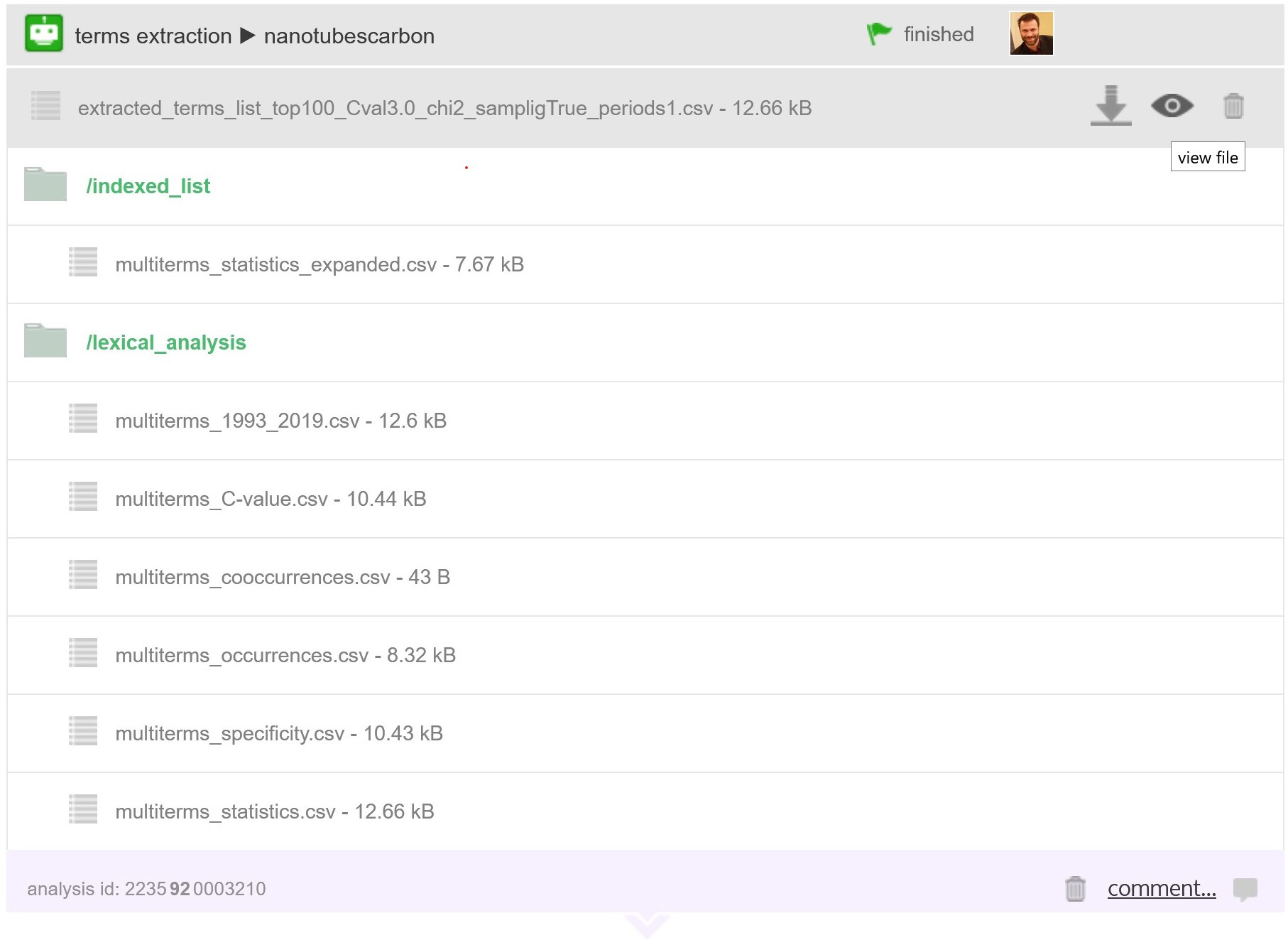
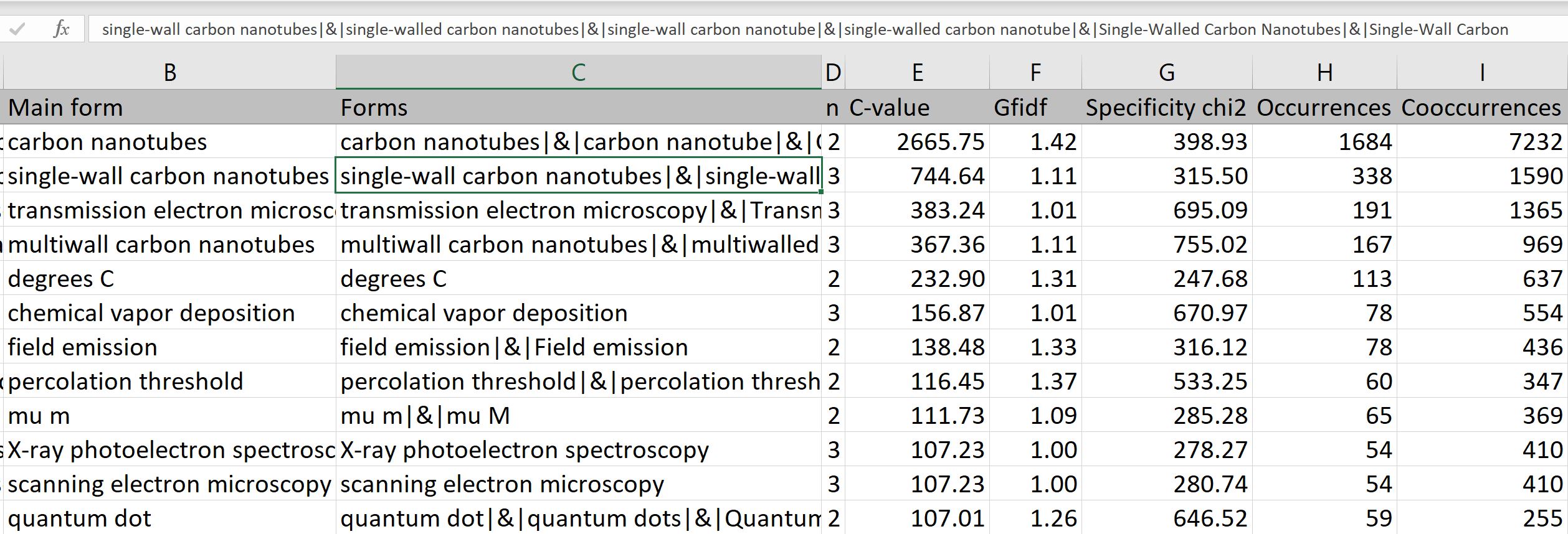
The first file (extracted_term_list…tsv) aggregate all statistic from all the periods, it includes all the extracted terms, where :

• Main form: is the selected main form of the list of forms. The main form will appear in the analyzes you will produced (using the terms variable or your custom indexation).
• Forms: all the indexed forms variations which appear in the textual variables selected, and correspond to the main form.

References

Kageura, K., & Umino, B. (1996). Methods of automatic term recognition: A review. Terminology. International Journal of Theoretical and Applied Issues in Specialized Communication, 3(2), 259-289.

Helmut Schmid (1995): Improvements in Part-of-Speech Tagging with an Application to German. Proceedings of the ACL SIGDAT-Workshop. Dublin, Ireland.

Helmut Schmid (1994): Probabilistic Part-of-Speech Tagging Using Decision Trees. Proceedings of International Conference on New Methods in Language Processing, Manchester, UK.

Frantzi, K. , Ananiadou S., & Mima H. (2000). Automatic recognition of multi-word terms:. the C-value/NC-value method, International Journal on Digital Libraries volume 3, pages 115–130

Porter, M. (1980). An algorithm for suffix stripping. Program, 14(3), 130–137.

Van Eck, N. J., & Waltman, L. (2011). Text mining and visualization using VOSviewer. Arxiv preprint arXiv:1109.2058.